机器学习sklearn19.0——线性回归算法(应用案例)_家庭用电预测——时间与有功功率之间的关系-程序员宅基地
技术标签: 机器学习
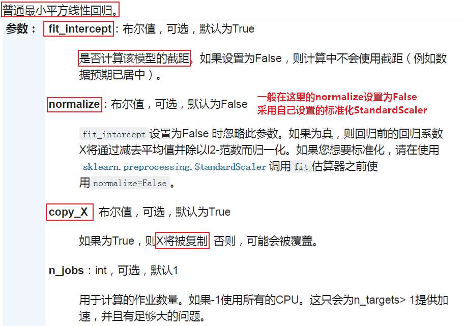
一、sklearn中的线性回归的使用


二、线性回归——家庭用电预测
(1)时间与功率之间的关系

#!/usr/bin/env python
# -*- coding:utf-8 -*-
# Author:ZhengzhengLiu
#线性回归——家庭用电预测(时间与功率之间的关系)
#导入模块
import sklearn
from sklearn.model_selection import train_test_split
from sklearn.linear_model import LinearRegression
from sklearn.preprocessing import StandardScaler
import numpy as np
import matplotlib as mpl
import matplotlib.pyplot as plt
import pandas as pd
from pandas import DataFrame
import time
#导入数据
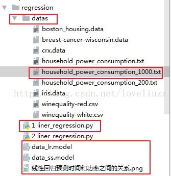
path = "datas/household_power_consumption_1000.txt"
data = pd.read_csv(path,sep=";")
#查看数据
print(data.head()) #查看头信息,默认前5行的数据
#iloc进行行列切片只能用数字下标,取出X的原始值(所有行与一、二列的表示时间的数据)
xdata = data.iloc[:,0:2]
# print(xdata)
y = data.iloc[:,2] #取出Y的数据(功率)
#y = data["Global_active_power"] #等价上面一句
# print(ydata)
#创建时间处理的函数
def time_format(x):
#join方法取出的两列数据用空格合并成一列
#用strptime方法将字符串形式的时间转换成时间元祖struct_time
t = time.strptime(" ".join(x), "%d/%m/%Y %H:%M:%S") #日月年时分秒的格式
# 分别返回年月日时分秒并放入到一个元组中
return (t.tm_year, t.tm_mon, t.tm_mday, t.tm_hour, t.tm_min, t.tm_sec)
#apply方法表示对xdata应用后面的转换形式
x = xdata.apply(lambda x:pd.Series(time_format(x)),axis=1)
print("======处理后的时间格式=======")
print(x.head())
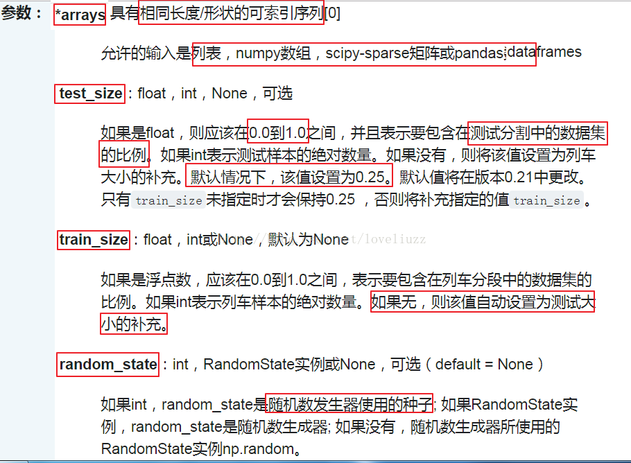
#划分测试集和训练集,random_state是随机数发生器使用的种子
x_train,x_test,y_train,y_test = train_test_split(x,y,test_size=0.3,random_state=1)
# print("========x_train=======")
# print(x_train)
# print("========x_text=======")
# print(x_test)
# print("========y_train=======")
# print(y_train)
# print("========y_text=======")
# print(y_test)
#对数据的训练集和测试集进行标准化
ss = StandardScaler()
#fit做运算,计算标准化需要的均值和方差;transform是进行转化
x_train = ss.fit_transform(x_train)
x_test = ss.transform(x_test)
#建立线性模型
lr = LinearRegression()
lr.fit(x_train,y_train) #训练
print("准确率:",lr.score(x_train,y_train)) #打印预测的决定系数,该值越接近于1越好
y_predict = lr.predict(x_test) #预测
# print(lr.score(x_text,y_predict))
#模型效果判断
mse = np.average((y_predict-np.array(y_test))**2)
rmse = np.sqrt(mse)
print("均方误差平方和:",mse)
print("均方误差平方和的平方根:",rmse)
#模型的保存与持久化
from sklearn.externals import joblib
joblib.dump(ss,"data_ss.model") #将标准化模型保存
joblib.dump(lr,"data_lr.model") #将训练后的线性模型保存
joblib.load("data_ss.model") #加载模型,会保存该model文件
joblib.load("data_lr.model") #加载模型
#预测值和实际值画图比较
#解决中文问题
mpl.rcParams["font.sans-serif"] = [u"SimHei"]
mpl.rcParams["axes.unicode_minus"] = False
t = np.arange(len(x_test))
plt.figure(facecolor="w") #创建画布,facecolor为背景色,w是白色(默认)
plt.plot(t,y_test,"r-",linewidth = 2,label = "真实值")
plt.plot(t,y_predict,"g-",linewidth = 2,label = "预测值")
plt.legend(loc = "upper right") #显示图例,设置图例的位置
plt.title("线性回归预测时间和功率之间的关系",fontsize=20)
plt.grid(b=True)
plt.savefig("线性回归预测时间和功率之间的关系.png") #保存图片
plt.show()
#运行结果:
Date Time Global_active_power Global_reactive_power Voltage \
0 16/12/2006 17:24:00 4.216 0.418 234.84
1 16/12/2006 17:25:00 5.360 0.436 233.63
2 16/12/2006 17:26:00 5.374 0.498 233.29
3 16/12/2006 17:27:00 5.388 0.502 233.74
4 16/12/2006 17:28:00 3.666 0.528 235.68
Global_intensity Sub_metering_1 Sub_metering_2 Sub_metering_3
0 18.4 0.0 1.0 17.0
1 23.0 0.0 1.0 16.0
2 23.0 0.0 2.0 17.0
3 23.0 0.0 1.0 17.0
4 15.8 0.0 1.0 17.0
======处理后的时间格式=======
0 1 2 3 4 5
0 2006 12 16 17 24 0
1 2006 12 16 17 25 0
2 2006 12 16 17 26 0
3 2006 12 16 17 27 0
4 2006 12 16 17 28 0
准确率: 0.232255807137
均方误差平方和: 1.18571330484
均方误差平方和的平方根: 1.08890463533

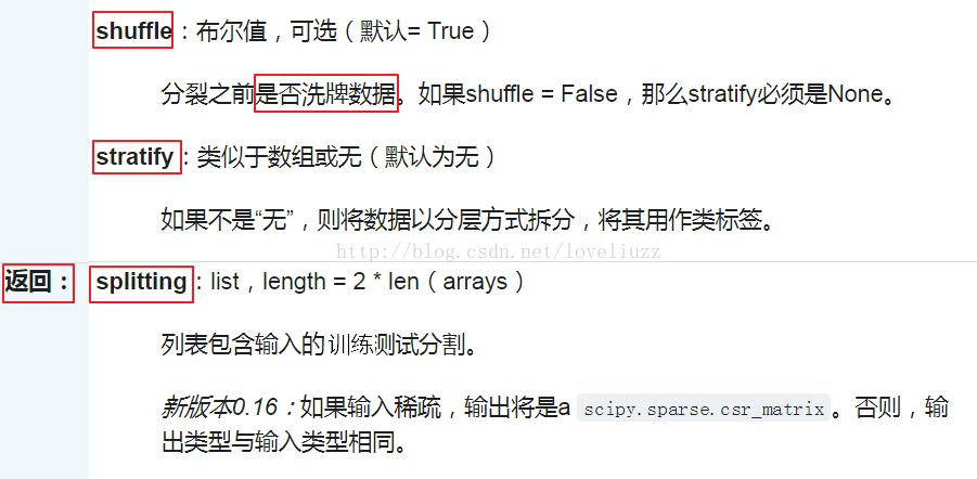
重要的模块——官方网站解释
1、train_test_split——划分测试集和训练集

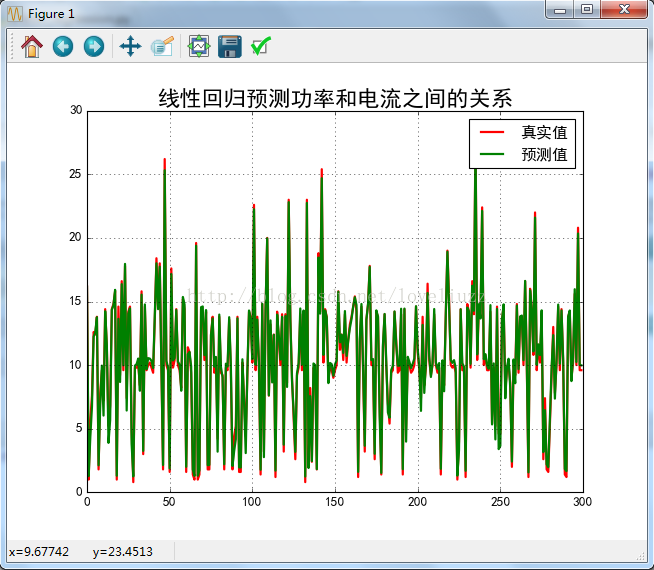
(2)线性回归——家庭用电预测(功率与电流之间的关系)
#!/usr/bin/env python
# -*- coding:utf-8 -*-
# Author:ZhengzhengLiu
#线性回归——家庭用电预测(功率与电压之间的关系)
#导入模块
import sklearn
from sklearn.model_selection import train_test_split
from sklearn.linear_model import LinearRegression
from sklearn.preprocessing import StandardScaler
import numpy as np
import matplotlib as mpl
import matplotlib.pyplot as plt
import pandas as pd
from pandas import DataFrame
#导入数据
path = "datas/household_power_consumption_1000.txt"
data = pd.read_csv(path,sep=";")
#iloc进行行列切片只能用数字下标,取出X的原始值(所有行与二、三列的表示功率的数据)
x = data.iloc[:,2:4]
y = data.iloc[:,5] #取出Y的数据(电流)
#划分训练集与测试集,random_state是随机数发生器使用的种子
x_train,x_test,y_train,y_test = train_test_split(x,y,test_size=0.3,random_state=1)
#对训练集和测试集进行标准化
ss = StandardScaler()
x_train = ss.fit_transform(x_train)
x_test = ss.transform(x_test)
#建立线性模型
lr = LinearRegression()
lr.fit(x_train,y_train) #训练
print("预测的决定系数R平方:",lr.score(x_train,y_train))
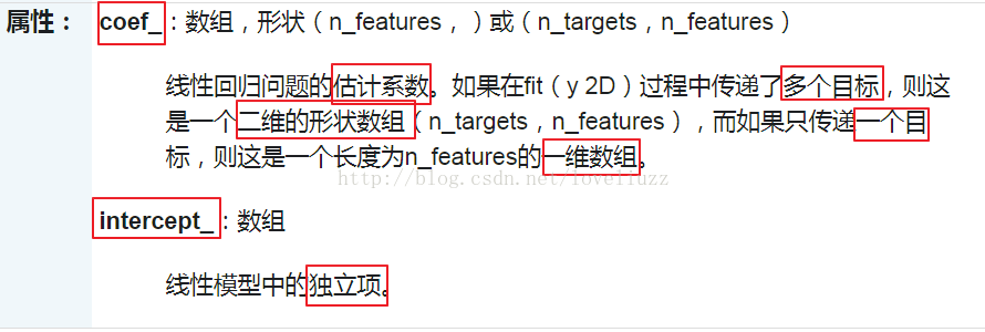
print("线性回归的估计系数:",lr.coef_) #打印线性回归的估计系数
print("线性模型的独立项:",lr.intercept_) #打印线性模型的独立项
y_predict = lr.predict(x_test) #预测
# print(y_predict)
#模型效果判断
mse = np.average((y_predict-np.array(y_test))**2)
rmse = np.sqrt(mse)
print("均方误差平方和:",mse)
print("均方误差平方和的平方根:",rmse)
#模型的保存与持久化
from sklearn.externals import joblib
joblib.dump(ss,"PI_data_ss.model") #将标准化模型保存
joblib.dump(lr,"PI_data_lr.model") #将训练后的线性模型保存
joblib.load("PI_data_ss.model") #加载模型,会保存该model文件
joblib.load("PI_data_lr.model") #加载模型
#预测值和实际值画图比较
#解决中文问题
mpl.rcParams["font.sans-serif"] = [u"SimHei"]
mpl.rcParams["axes.unicode_minus"] = False
p = np.arange(len(x_test))
plt.figure(facecolor="w") #创建画布,facecolor为背景色,w是白色
plt.plot(p,y_test,"r-",linewidth = 2,label = "真实值")
plt.plot(p,y_predict,"g-",linewidth = 2,label = "预测值")
plt.legend(loc = "upper right") #显示图例,设置图例的位置
plt.title("线性回归预测功率和电流之间的关系",fontsize = 20)
plt.grid(b=True)
plt.savefig("线性回归预测功率和电流之间的关系.png")
plt.show()
#运行结果:
预测的决定系数R平方: 0.990719383392
线性回归的估计系数: [ 5.12959849 0.0589354 ]
线性模型的独立项: 10.3485714286
均方误差平方和: 0.193026891251
均方误差平方和的平方根: 0.439348257366
(3)线性回归——家庭用电预测(时间与电压之间的多项式关系)
#!/usr/bin/env python
# -*- coding:utf-8 -*-
# Author:ZhengzhengLiu

#线性回归——家庭用电预测(时间与电压之间的多项式关系)

import sklearn
from sklearn.model_selection import train_test_split
from sklearn.linear_model import LinearRegression,Lasso,Ridge
from sklearn.preprocessing import StandardScaler
from sklearn.preprocessing import PolynomialFeatures    #多项式
from sklearn.pipeline import Pipeline
from sklearn.model_selection import GridSearchCV    #带有交叉验证的网格搜索

import numpy as np
import matplotlib as mpl
import matplotlib.pyplot as plt
import pandas as pd
import time

#创建时间处理的函数
def time_format(x):
    #join方法取出的两列数据用空格合并成一列
    #用strptime方法将字符串形式的时间转换成时间元祖struct_time
    t = time.strptime(" ".join(x), "%d/%m/%Y %H:%M:%S")   #日月年时分秒的格式
    # 分别返回年月日时分秒并放入到一个元组中
    return (t.tm_year, t.tm_mon, t.tm_mday, t.tm_hour, t.tm_min, t.tm_sec)

#解决中文问题
mpl.rcParams["font.sans-serif"] = [u"SimHei"]
mpl.rcParams["axes.unicode_minus"] = False

#导入数据
path = "datas/household_power_consumption_1000.txt"
data = pd.read_csv(path,sep=";",low_memory=False)

#日期,时间,有功功率,无功功率,电压,电流,厨房用电功率,洗衣服用电功率,热水器用电功率

names = ['Date','Time','Global_active_power','Global_reactive_power','Voltage','Global_intensity','Sub_metering_1','Sub_metering_2','Sub_metering_3']

#异常数据处理(异常数据过滤)
new_data = data.replace("?",np.nan)
datas = new_data.dropna(axis=0, how="any")       #只要有数据为空就进行行删除操作

#时间与电压之间的关系(Liner--多项式)
models = [
    Pipeline([
        ('Poly',PolynomialFeatures()),
        ('Linear',LinearRegression(fit_intercept=False))
    ])
]

model = models[0]

#获取x和y变量,并将时间转换成数值连续型变量
xdata = data.iloc[:,0:2]
x = xdata.apply(lambda x:pd.Series(time_format(x)),axis=1)  #apply方法表示对xdata应用后面的转换形式
y = data.iloc[:,4]      #取出Y的数据(电压)

#划分测试集和训练集,random_state是随机数发生器使用的种子
x_train,x_test,y_train,y_test = train_test_split(x,y,test_size=0.3,random_state=0)

#对数据的训练集和测试集进行标准化
ss = StandardScaler()
#fit做运算,计算标准化需要的均值和方差;transform是进行转化
x_train = ss.fit_transform(x_train)
x_test = ss.transform(x_test)

#模型训练
t = np.arange(len(x_test))
N = 5
d_pool = np.arange(1,N,1)   #阶
m = d_pool.size
clrs = []       #颜色
for c in np.linspace(16711680,255,m):
    clrs.append('#%06x' % int(c))
line_width = 3

plt.figure(figsize=(12,6),facecolor='w')    #创建绘图窗口,设置大小和背景颜色
for i,d in enumerate(d_pool):
    plt.subplot(N-1,1,i+1)
    plt.plot(t,y_test,"r-",label = "真实值",ms = 10,zorder=N)
    model.set_params(Poly__degree=d)    #set_params函数对Pipeline中的某个模型设置参数
    model.fit(x_train,y_train)
    lin = model.get_params('Linear')['Linear']
    output = u"%d阶,系数为:" % d
    print(output, lin.coef_.ravel())  # ravel方法将数组拉直,多维数组将为一维

    y_hat = model.predict(x_test)
    s = model.score(x_test,y_test)
    z = N-1 if (d==2) else 0
    label = u"%d阶,准确率为:%.3f" % (d, s)
    plt.plot(t, y_hat, color=clrs[i], lw=line_width, alpha=0.75, label=label, zorder=z)
    plt.legend(loc="upper left")
    plt.grid(True)
    plt.ylabel(u"%d阶结果" % d, fontsize=12)

plt.legend(loc="lower right")
plt.suptitle(u"线性回归预测时间与电压之间的多项式关系",fontsize=20)
plt.grid(True)
plt.show()

#运行结果:
1阶,系数为: [  2.39902814e+02   0.00000000e+00   1.11022302e-16   4.23207026e+00
   1.12142760e+00   2.02166226e-01   0.00000000e+00]
2阶,系数为: [ -1.11539792e+13   2.92968750e-03  -6.83593750e-03   4.14912590e+12
   3.23876953e+00   3.21350098e-01   7.99560547e-03   2.44140625e-04
   0.00000000e+00   0.00000000e+00   0.00000000e+00   0.00000000e+00
   0.00000000e+00   0.00000000e+00   0.00000000e+00   0.00000000e+00
   0.00000000e+00   0.00000000e+00   1.11539792e+13  -2.54700928e+01
  -6.71875000e-01   0.00000000e+00  -1.03660889e+01  -5.82519531e-01
   0.00000000e+00  -8.44726562e-02   0.00000000e+00   0.00000000e+00]
3阶,系数为: [ -1.63002196e+13  -1.06171697e+12  -2.19799440e+13   2.68220670e+13
  -2.01883991e+13   1.17965159e+13   4.59169674e+12   1.33751216e+13
  -7.30563919e+11   2.49935263e+12  -3.41816728e+12   4.70268465e+12
   3.41993070e+12   4.34249277e+12  -2.36933344e+12   1.99575089e+12
   1.66261330e+12   0.00000000e+00   8.57830362e+12   7.50980509e+12
  -4.38814065e+12   0.00000000e+00   7.84667969e-01   1.88476562e-01
   0.00000000e+00  -4.19921875e-02   0.00000000e+00   0.00000000e+00
   0.00000000e+00   0.00000000e+00   0.00000000e+00   0.00000000e+00
   0.00000000e+00   0.00000000e+00   0.00000000e+00   0.00000000e+00
   0.00000000e+00   0.00000000e+00   0.00000000e+00   0.00000000e+00
   0.00000000e+00   0.00000000e+00   0.00000000e+00   0.00000000e+00
   0.00000000e+00   0.00000000e+00   0.00000000e+00   0.00000000e+00
   0.00000000e+00   0.00000000e+00   0.00000000e+00   0.00000000e+00
   0.00000000e+00   0.00000000e+00   0.00000000e+00   0.00000000e+00
   0.00000000e+00   0.00000000e+00   0.00000000e+00   0.00000000e+00
   0.00000000e+00   0.00000000e+00   0.00000000e+00   0.00000000e+00
  -2.07586109e+13   2.01883991e+13  -1.17965159e+13   0.00000000e+00
  -7.69610596e+00  -5.44921875e-01   0.00000000e+00  -8.59375000e-02
   0.00000000e+00   0.00000000e+00   3.87646484e+00   2.26562500e-01
   0.00000000e+00  -1.87500000e-01   0.00000000e+00   0.00000000e+00
  -2.16796875e-01   0.00000000e+00   0.00000000e+00   0.00000000e+00]
4阶,系数为: [ -6.00682517e+11  -3.29239328e+12   1.86141729e+13   6.93021510e+11
   2.69953823e+12  -6.17642085e+11  -2.70513938e+12  -1.02422258e+12
   1.91156682e+12  -7.75735474e+11  -1.00006158e+12  -3.39208470e+11
   5.77229194e+11   4.27298991e+11  -1.07091942e+12   4.84607019e+11
   2.02165069e+12   8.34755567e+10   8.99308537e+12  -9.15830049e+12
  -5.29757907e+11  -8.45993774e+10   9.23510075e+12  -6.18929887e+11
   3.35305892e+10   8.50306093e+12  -7.26209570e+10  -1.36507996e+10
   1.00507638e+10   0.00000000e+00   0.00000000e+00   0.00000000e+00
   0.00000000e+00   0.00000000e+00   0.00000000e+00   0.00000000e+00
   0.00000000e+00   0.00000000e+00   0.00000000e+00   0.00000000e+00
   0.00000000e+00   0.00000000e+00   0.00000000e+00   0.00000000e+00
   0.00000000e+00   0.00000000e+00   0.00000000e+00   0.00000000e+00
   0.00000000e+00   0.00000000e+00   0.00000000e+00   0.00000000e+00
   0.00000000e+00   0.00000000e+00   0.00000000e+00   0.00000000e+00
   0.00000000e+00   0.00000000e+00   0.00000000e+00   0.00000000e+00
   0.00000000e+00   0.00000000e+00   0.00000000e+00   0.00000000e+00
  -3.65641060e+12   3.33677698e+11   9.00170118e+11   0.00000000e+00
  -3.43532967e+12   2.30233352e+11   0.00000000e+00  -3.16302099e+12
   0.00000000e+00   0.00000000e+00  -1.65683594e+01  -1.81250000e+00
   0.00000000e+00  -3.91601562e-01   0.00000000e+00   0.00000000e+00
  -2.19726562e-01   0.00000000e+00   0.00000000e+00   0.00000000e+00
   0.00000000e+00   0.00000000e+00   0.00000000e+00   0.00000000e+00
   0.00000000e+00   0.00000000e+00   0.00000000e+00   0.00000000e+00
   0.00000000e+00   0.00000000e+00   0.00000000e+00   0.00000000e+00
   0.00000000e+00   0.00000000e+00   0.00000000e+00   0.00000000e+00
   0.00000000e+00   0.00000000e+00   0.00000000e+00   0.00000000e+00
   0.00000000e+00   0.00000000e+00   0.00000000e+00   0.00000000e+00
   0.00000000e+00   0.00000000e+00   0.00000000e+00   0.00000000e+00
   0.00000000e+00   0.00000000e+00   0.00000000e+00   0.00000000e+00
   0.00000000e+00   0.00000000e+00   0.00000000e+00   0.00000000e+00
   0.00000000e+00   0.00000000e+00   0.00000000e+00   0.00000000e+00
   0.00000000e+00   0.00000000e+00   0.00000000e+00   0.00000000e+00
   0.00000000e+00   0.00000000e+00   0.00000000e+00   0.00000000e+00
   0.00000000e+00   0.00000000e+00   0.00000000e+00   0.00000000e+00
   0.00000000e+00   0.00000000e+00   0.00000000e+00   0.00000000e+00
   0.00000000e+00   0.00000000e+00   0.00000000e+00   0.00000000e+00
   0.00000000e+00   0.00000000e+00   0.00000000e+00   0.00000000e+00
   0.00000000e+00   0.00000000e+00   0.00000000e+00   0.00000000e+00
   0.00000000e+00   0.00000000e+00   0.00000000e+00   0.00000000e+00
   0.00000000e+00   0.00000000e+00   0.00000000e+00   0.00000000e+00
   0.00000000e+00   0.00000000e+00   0.00000000e+00   0.00000000e+00
   0.00000000e+00   0.00000000e+00   0.00000000e+00   0.00000000e+00
   0.00000000e+00   0.00000000e+00   0.00000000e+00   0.00000000e+00
   0.00000000e+00   0.00000000e+00   0.00000000e+00  -8.56707860e+12
   8.15410963e+12   7.59512214e+11   0.00000000e+00  -9.23510075e+12
   6.18929887e+11   0.00000000e+00  -8.50306093e+12   0.00000000e+00
   0.00000000e+00  -3.61572266e-01  -8.24658203e+00   0.00000000e+00
  -7.02392578e-01   0.00000000e+00   0.00000000e+00  -7.81250000e-02
   0.00000000e+00   0.00000000e+00   0.00000000e+00  -7.55639648e+00
  -3.84765625e+00   0.00000000e+00  -5.38574219e-01   0.00000000e+00
   0.00000000e+00   1.22070312e-01   0.00000000e+00   0.00000000e+00
   0.00000000e+00   1.22070312e-02   0.00000000e+00   0.00000000e+00
   0.00000000e+00   0.00000000e+00]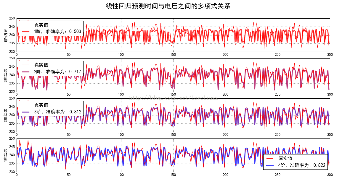
4、过拟合样例代码以及几种算法的多项式过拟合比较
#!/usr/bin/env python
# -*- coding:utf-8 -*-
# Author:ZhengzhengLiu

#过拟合样例代码
import sklearn
from sklearn.preprocessing import PolynomialFeatures
from sklearn.pipeline import Pipeline
from sklearn.linear_model import LinearRegression,LassoCV,RidgeCV,ElasticNetCV
from sklearn.linear_model.coordinate_descent import ConvergenceWarning

import numpy as np
import pandas as pd
import matplotlib as mpl
import matplotlib.pyplot as plt
import warnings

#解决中文问题
mpl.rcParams["font.sans-serif"] = [u"SimHei"]
mpl.rcParams["axes.unicode_minus"] = False

np.random.seed(100)     #seed() 设置生成随机数用的整数起始值
np.set_printoptions(linewidth=1000,suppress=True)
N  =10
x = np.linspace(0,6,N)+np.random.randn(N)
y = 1.8*x**3+x**2-14*x-7+np.random.randn(N)

x.shape = -1,1      #转完成一列
y.shape = -1,1

models = [
    Pipeline([
        ('Poly',PolynomialFeatures()),
        ('Linear',LinearRegression(fit_intercept=False))
    ]),
    Pipeline([
        ('Poly',PolynomialFeatures()),
        ('Linear',RidgeCV(alphas=np.logspace(-3,2,50),fit_intercept=False))
    ]),
    Pipeline([
        ('Poly',PolynomialFeatures()),
        ('Linear',LassoCV(alphas=np.logspace(-3,2,50),fit_intercept=False))
    ]),
    Pipeline([
        ('Poly',PolynomialFeatures()),
        ('Linear',ElasticNetCV(alphas=np.logspace(-3,2,50),l1_ratio=[.1,.5,.7,.9,.95,1],fit_intercept=False))
    ])
]

plt.figure(facecolor='w')   #创建画布
degree = np.arange(1,N,4)   #阶数(一阶,五阶,九阶)
dm = degree.size
colors = []
for c in np.linspace(16711680,255,dm):
    c = c.astype(int)
    colors.append('#%06x' % c)

model = models[0]

for i,d in enumerate(degree):
    plt.subplot(int(np.ceil(dm/2.0)),2,i+1)
    plt.plot(x,y,'ro',ms=10,zorder=N)

    model.set_params(Poly__degree=d)
    model.fit(x,y.ravel())

    lin = model.get_params('Linear')['Linear']
    output = u'%d阶,系数为' %d
    print(output,lin.coef_.ravel())

    x_hat = np.linspace(x.min(),x.max(),num=100)
    x_hat.shape = -1,1
    y_hat = model.predict(x_hat)
    s = model.score(x,y)

    z = N-1 if (d==2) else 0
    label = u"%d阶,准确率为:%.3f" % (d, s)
    plt.plot(x_hat, y_hat, color=colors[i], lw=2, alpha=0.75, label=label, zorder=z)

    plt.legend(loc="upper left")
    plt.grid(True)
    plt.xlabel('X', fontsize=16)
    plt.ylabel('Y', fontsize=16)

plt.tight_layout(1,rect=(0,0,1,0.95))
plt.suptitle(u'线性回归过拟合显示',fontsize=22)
plt.savefig('线性回归过拟合显示.png')
plt.show()

#运行结果:
1阶,系数为 [-44.14102611  40.05964256]
5阶,系数为 [ -5.60899679 -14.80109301   0.75014858   2.11170671  -0.07724668   0.00566633]
9阶,系数为 [-2465.5996245   6108.67810881 -5112.02743837   974.75680049  1078.90344647  -829.50835134   266.13413535   -45.7177359      4.11585669    -0.15281174]
#!/usr/bin/env python
# -*- coding:utf-8 -*-
# Author:ZhengzhengLiu

#几种算法的多项式过拟合比较
import sklearn
from sklearn.preprocessing import PolynomialFeatures
from sklearn.pipeline import Pipeline
from sklearn.linear_model import LinearRegression,LassoCV,RidgeCV,ElasticNetCV
from sklearn.linear_model.coordinate_descent import ConvergenceWarning

import numpy as np
import pandas as pd
import matplotlib as mpl
import matplotlib.pyplot as plt
import warnings

#解决中文问题
mpl.rcParams["font.sans-serif"] = [u"SimHei"]
mpl.rcParams["axes.unicode_minus"] = False

np.random.seed(100)     #seed() 设置生成随机数用的整数起始值
np.set_printoptions(linewidth=1000,suppress=True)
N  =10
x = np.linspace(0,6,N)+np.random.randn(N)
y = 1.8*x**3+x**2-14*x-7+np.random.randn(N)

x.shape = -1,1      #转完成一列
y.shape = -1,1

models = [
    Pipeline([
        ('Poly',PolynomialFeatures()),
        ('Linear',LinearRegression(fit_intercept=False))
    ]),
    Pipeline([
        ('Poly',PolynomialFeatures()),
        ('Linear',RidgeCV(alphas=np.logspace(-3,2,50),fit_intercept=False))
    ]),
    Pipeline([
        ('Poly',PolynomialFeatures()),
        ('Linear',LassoCV(alphas=np.logspace(-3,2,50),fit_intercept=False))
    ]),
    Pipeline([
        ('Poly',PolynomialFeatures()),
        ('Linear',ElasticNetCV(alphas=np.logspace(-3,2,50),l1_ratio=[.1,.5,.7,.9,.95,1],fit_intercept=False))
    ])
]

plt.figure(facecolor='w')
degree = np.arange(1, N, 2)  # 阶
dm = degree.size
colors = []  # 颜色
for c in np.linspace(16711680, 255, dm):
    c = c.astype(int)
    colors.append('#%06x' % c)
titles = [u'线性回归', u'Ridge回归', u'Lasso回归', u'ElasticNet']

for t in range(4):
    model = models[t]
    plt.subplot(2, 2, t + 1)
    plt.plot(x, y, 'ro', ms=10, zorder=N)

    for i, d in enumerate(degree):
        model.set_params(Poly__degree=d)

        model.fit(x, y.ravel())

        lin = model.get_params('Linear')['Linear']

        output = u'%s:%d阶,系数为:' % (titles[t], d)
        print(output, lin.coef_.ravel())

        x_hat = np.linspace(x.min(), x.max(), num=100)
        x_hat.shape = -1, 1

        y_hat = model.predict(x_hat)

        s = model.score(x, y)

        z = N - 1 if (d == 2) else 0
        label = u'%d阶, 正确率=%.3f' % (d, s)
        plt.plot(x_hat, y_hat, color=colors[i], lw=2, alpha=0.75, label=label, zorder=z)

    plt.legend(loc='upper left')
    plt.grid(True)
    plt.title(titles[t])
    plt.xlabel('X', fontsize=16)
    plt.ylabel('Y', fontsize=16)
plt.tight_layout(1, rect=(0, 0, 1, 0.95))
plt.suptitle(u'各种不同线性回归过拟合显示', fontsize=22)
plt.savefig('各种不同线性回归过拟合显示.png')
plt.show()

#运行结果:
线性回归:1阶,系数为: [-44.14102611  40.05964256]
线性回归:3阶,系数为: [ -6.80525963 -13.743068     0.93453895   1.79844791]
线性回归:5阶,系数为: [ -5.60899679 -14.80109301   0.75014858   2.11170671  -0.07724668   0.00566633]
线性回归:7阶,系数为: [-41.70721173  52.3857053  -29.56451339  -7.6632283   12.07162703  -3.86969096   0.53286096  -0.02725536]
线性回归:9阶,系数为: [-2465.59964345  6108.67815659 -5112.02747906   974.75680883  1078.9034548   -829.50835799   266.13413753   -45.71773628     4.11585673    -0.15281174]
Ridge回归:1阶,系数为: [ -6.71593385  29.79090057]
Ridge回归:3阶,系数为: [ -6.7819845  -13.73679293   0.92827639   1.79920954]
Ridge回归:5阶,系数为: [-0.82920155 -1.07244754 -1.41803017 -0.93057536  0.88319116 -0.07073168]
Ridge回归:7阶,系数为: [-1.62586368 -2.18512108 -1.82690987 -2.27495708  0.98685071  0.30551091 -0.10988434  0.00846908]
Ridge回归:9阶,系数为: [-10.50566712  -6.12564342  -1.96421973   0.80200162   0.59148105  -0.23358229   0.20297054  -0.08109453   0.01327453  -0.00061892]
Lasso回归:1阶,系数为: [ -0.          29.27359177]
Lasso回归:3阶,系数为: [ -6.7688595  -13.75928024   0.93989323   1.79778598]
Lasso回归:5阶,系数为: [ -0.         -12.00109345  -0.50746853   1.74395236   0.07086952  -0.00583605]
Lasso回归:7阶,系数为: [-0.         -0.         -0.         -0.08083315  0.19550746  0.03066137 -0.00020584 -0.00046928]
Lasso回归:9阶,系数为: [-0.         -0.         -0.         -0.          0.04439727  0.05587113  0.00109023 -0.00021498 -0.00004479 -0.00000674]
ElasticNet:1阶,系数为: [-13.22089654  32.08359338]
ElasticNet:3阶,系数为: [ -6.7688595  -13.75928024   0.93989323   1.79778598]
ElasticNet:5阶,系数为: [-1.65823671 -5.20271875 -1.26488859  0.94503683  0.2605984  -0.01683786]
ElasticNet:7阶,系数为: [-0.         -0.         -0.         -0.15812511  0.22150166  0.02955069 -0.00040066 -0.00046568]
ElasticNet:9阶,系数为: [-0.         -0.         -0.         -0.          0.05255118  0.05364699  0.00111995 -0.00020596 -0.00004365 -0.00000667]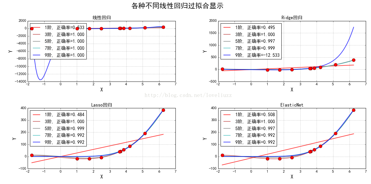
智能推荐
攻防世界_难度8_happy_puzzle_攻防世界困难模式攻略图文-程序员宅基地
文章浏览阅读645次。这个肯定是末尾的IDAT了,因为IDAT必须要满了才会开始一下个IDAT,这个明显就是末尾的IDAT了。,对应下面的create_head()代码。,对应下面的create_tail()代码。不要考虑爆破,我已经试了一下,太多情况了。题目来源:UNCTF。_攻防世界困难模式攻略图文
达梦数据库的导出(备份)、导入_达梦数据库导入导出-程序员宅基地
文章浏览阅读2.9k次,点赞3次,收藏10次。偶尔会用到,记录、分享。1. 数据库导出1.1 切换到dmdba用户su - dmdba1.2 进入达梦数据库安装路径的bin目录,执行导库操作 导出语句:./dexp cwy_init/[email protected]:5236 file=cwy_init.dmp log=cwy_init_exp.log 注释: cwy_init/init_123..._达梦数据库导入导出
js引入kindeditor富文本编辑器的使用_kindeditor.js-程序员宅基地
文章浏览阅读1.9k次。1. 在官网上下载KindEditor文件,可以删掉不需要要到的jsp,asp,asp.net和php文件夹。接着把文件夹放到项目文件目录下。2. 修改html文件,在页面引入js文件:<script type="text/javascript" src="./kindeditor/kindeditor-all.js"></script><script type="text/javascript" src="./kindeditor/lang/zh-CN.js"_kindeditor.js
STM32学习过程记录11——基于STM32G431CBU6硬件SPI+DMA的高效WS2812B控制方法-程序员宅基地
文章浏览阅读2.3k次,点赞6次,收藏14次。SPI的详情简介不必赘述。假设我们通过SPI发送0xAA,我们的数据线就会变为10101010,通过修改不同的内容,即可修改SPI中0和1的持续时间。比如0xF0即为前半周期为高电平,后半周期为低电平的状态。在SPI的通信模式中,CPHA配置会影响该实验,下图展示了不同采样位置的SPI时序图[1]。CPOL = 0,CPHA = 1:CLK空闲状态 = 低电平,数据在下降沿采样,并在上升沿移出CPOL = 0,CPHA = 0:CLK空闲状态 = 低电平,数据在上升沿采样,并在下降沿移出。_stm32g431cbu6
计算机网络-数据链路层_接收方收到链路层数据后,使用crc检验后,余数为0,说明链路层的传输时可靠传输-程序员宅基地
文章浏览阅读1.2k次,点赞2次,收藏8次。数据链路层习题自测问题1.数据链路(即逻辑链路)与链路(即物理链路)有何区别?“电路接通了”与”数据链路接通了”的区别何在?2.数据链路层中的链路控制包括哪些功能?试讨论数据链路层做成可靠的链路层有哪些优点和缺点。3.网络适配器的作用是什么?网络适配器工作在哪一层?4.数据链路层的三个基本问题(帧定界、透明传输和差错检测)为什么都必须加以解决?5.如果在数据链路层不进行帧定界,会发生什么问题?6.PPP协议的主要特点是什么?为什么PPP不使用帧的编号?PPP适用于什么情况?为什么PPP协议不_接收方收到链路层数据后,使用crc检验后,余数为0,说明链路层的传输时可靠传输
软件测试工程师移民加拿大_无证移民,未受过软件工程师的教育(第1部分)-程序员宅基地
文章浏览阅读587次。软件测试工程师移民加拿大 无证移民,未受过软件工程师的教育(第1部分) (Undocumented Immigrant With No Education to Software Engineer(Part 1))Before I start, I want you to please bear with me on the way I write, I have very little gen...
随便推点
Thinkpad X250 secure boot failed 启动失败问题解决_安装完系统提示secureboot failure-程序员宅基地
文章浏览阅读304次。Thinkpad X250笔记本电脑,装的是FreeBSD,进入BIOS修改虚拟化配置(其后可能是误设置了安全开机),保存退出后系统无法启动,显示:secure boot failed ,把自己惊出一身冷汗,因为这台笔记本刚好还没开始做备份.....根据错误提示,到bios里面去找相关配置,在Security里面找到了Secure Boot选项,发现果然被设置为Enabled,将其修改为Disabled ,再开机,终于正常启动了。_安装完系统提示secureboot failure
C++如何做字符串分割(5种方法)_c++ 字符串分割-程序员宅基地
文章浏览阅读10w+次,点赞93次,收藏352次。1、用strtok函数进行字符串分割原型: char *strtok(char *str, const char *delim);功能:分解字符串为一组字符串。参数说明:str为要分解的字符串,delim为分隔符字符串。返回值:从str开头开始的一个个被分割的串。当没有被分割的串时则返回NULL。其它:strtok函数线程不安全,可以使用strtok_r替代。示例://借助strtok实现split#include <string.h>#include <stdio.h&_c++ 字符串分割
2013第四届蓝桥杯 C/C++本科A组 真题答案解析_2013年第四届c a组蓝桥杯省赛真题解答-程序员宅基地
文章浏览阅读2.3k次。1 .高斯日记 大数学家高斯有个好习惯:无论如何都要记日记。他的日记有个与众不同的地方,他从不注明年月日,而是用一个整数代替,比如:4210后来人们知道,那个整数就是日期,它表示那一天是高斯出生后的第几天。这或许也是个好习惯,它时时刻刻提醒着主人:日子又过去一天,还有多少时光可以用于浪费呢?高斯出生于:1777年4月30日。在高斯发现的一个重要定理的日记_2013年第四届c a组蓝桥杯省赛真题解答
基于供需算法优化的核极限学习机(KELM)分类算法-程序员宅基地
文章浏览阅读851次,点赞17次,收藏22次。摘要:本文利用供需算法对核极限学习机(KELM)进行优化,并用于分类。
metasploitable2渗透测试_metasploitable2怎么进入-程序员宅基地
文章浏览阅读1.1k次。一、系统弱密码登录1、在kali上执行命令行telnet 192.168.26.1292、Login和password都输入msfadmin3、登录成功,进入系统4、测试如下:二、MySQL弱密码登录:1、在kali上执行mysql –h 192.168.26.129 –u root2、登录成功,进入MySQL系统3、测试效果:三、PostgreSQL弱密码登录1、在Kali上执行psql -h 192.168.26.129 –U post..._metasploitable2怎么进入
Python学习之路:从入门到精通的指南_python人工智能开发从入门到精通pdf-程序员宅基地
文章浏览阅读257次。本文将为初学者提供Python学习的详细指南,从Python的历史、基础语法和数据类型到面向对象编程、模块和库的使用。通过本文,您将能够掌握Python编程的核心概念,为今后的编程学习和实践打下坚实基础。_python人工智能开发从入门到精通pdf