G2O，与ceres并列为目前视觉SLAM中应用最广泛的优化算法库。它最大的特点就是基于图优化设计，这对于视觉SLAM来说是异常适配的。在很多的SLAM库的中都使用到它来进行优化操作，比如ORB-SLAM。

代码仓库：https://github.com/RainerKuemmerle/g2o。

本文所对照的源码版本是2023.9.1日期，因此和网上其他的一些教程版本有些出入，但是总体相差不大。总体来说，差别在BlockSolver的接口由裸指针变成了unique_ptr、VertexSBAPointXYZ类被删除等。具体可以看：SLAM十四讲ch7代码调整（undefined reference to symbol）。

G2O库简介

G2O的全称为：General Graphic Optimization，通用图优化。为何叫通用呢？

G2O的核里带有各种各样的求解器，而它的顶点、边的类型则多种多样。通过自定义顶点和边，事实上，只要一个优化问题能够表达成图，那么就可以用G2O去求解它。常见的，比如bundle adjustment、ICP、数据拟合，都可以用G2O来做。

所谓图优化，是把优化问题表现成图的一种方式，这里的图是图论意义上的图。一个图由若干个顶点，以及连着这些顶点的边组成。在这里，我们用顶点表示优化变量，而用边表示残差项。

下图展示的就是一些优化问题的图的表现形式，左图是诸如曲线拟合等一元边，右图是诸如BA等二元边的情况：

G2O使用流程

下图是G2O的基础框架结构，它几乎包含了所有重要的类之间的关系：

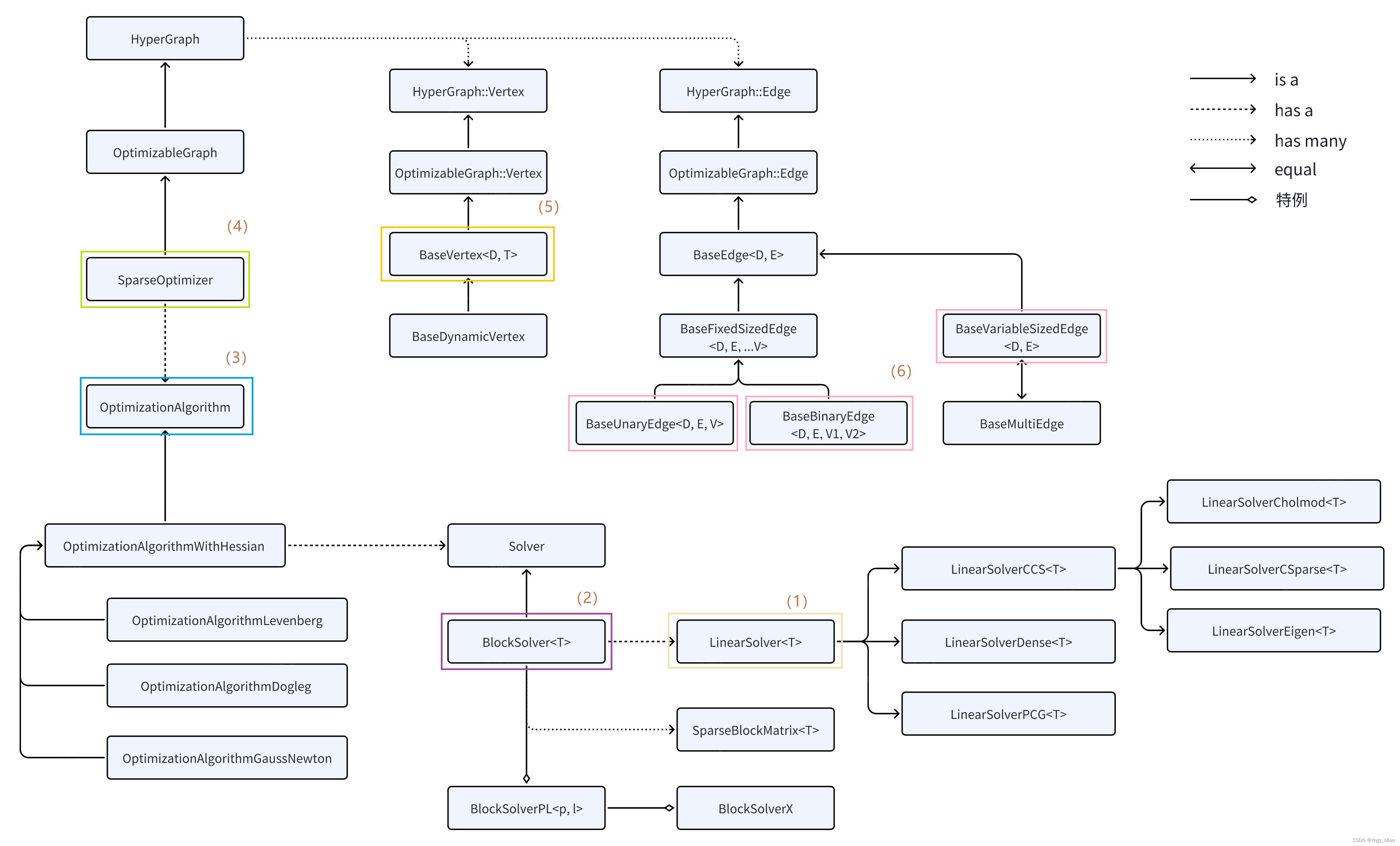
其中：

• SparseOptimizer：稀疏优化器，它有基类OptimizableGraph（可优化图），又有基类HyperGraph（超图）
• Vertex：顶点，它是图的数据成员，会有很多定制化的子类
• Edge：边，它是图的数据成员，会有很多定制化的子类
• OptimizationAlgorithm：优化算法，它是图的数据成员，可以指定Gauss-Newton、Levernberg-Marquardt、Powell’s dogleg等迭代算法
• Solver：求解器，它是优化算法的数据成员，它有两个部分，计算稀疏（Schur舒尔补）的雅可比和Hessian矩阵（SparseBlockMatrix），计算迭代过程中最关键的一步 $H\Delta x=-b$（LinearSolver）

从顶层到底层梳理完整个的基础框架结构，在编程实现时需要反过来，从底层开始搭建框架一直到顶层：

1. 【STEP1】构建一个优化求解器LinearSolver、BlockSolver、OptimizationAlgorithm

2. 【STEP2】构建稀疏优化器SparseOptimizer

3. 【STEP3】定义并添加图的顶点Vertex、边Edge

4. 【STEP4】设置优化参数，开始执行优化

一个简单的代码实现是：

typedef g2o::BlockSolver<g2o::BlockSolverTraits<3, 1> > Block;  // 待优化变量维度为3，测量值维度为1

// STEP1：构建优化求解器
std::unique_ptr<Block::LinearSolverType> linearSolver(new g2o::LinearSolverCSparse<Block::PoseMatrixType>());
std::unique_ptr<Block> solver_ptr(new Block(std::move(linearSolver)));
g2o::OptimizationAlgorithmLevenberg* solver = new g2o::OptimizationAlgorithmLevenberg(std::move(solver_ptr));

// STEP2：构建稀疏优化器
g2o::SparseOptimizer optimizer;
optimizer.setAlgorithm(solver);   // 设置求解器
optimizer.setVerbose(true);       // 打开调试输出

// STEP3：定义并添加图的顶点、边
optimizer.addVertex(new MyVertex());
optimizer.addEdge(new MyEdge());

// STEP4：设置优化参数，开始执行优化
optimizer.initializeOptimization();
optimizer.optimize(100);

下面将会对其中的重要的几个STEP进行详细讲解。

构建优化求解器（STEP1）

求解器的有三种：LinearSolver、BlockSolver、OptimizationAlgorithm。

线性求解器LinearSolver

由于在迭代的过程中，基本都需要求解近似于 $H\Delta x=-b$ 的增量方程。

通常情况下想到的方法就是直接求逆，也就是 $\Delta x=-H^{-1}b$。看起来好像很简单，但这有个前提，就是H的维度较小，此时只需要矩阵的求逆就能解决问题。但是当H的维度较大时，矩阵求逆变得很困难，求解问题也变得很复杂。

因此，G2O提供了各种求解该线性方程的线性求解器，这里就直接总结一下几种预设：

// 使用sparse cholesky分解法
LinearSolverCholmod : public LinearSolverCCS<MatrixType>;
// 依赖项只有eigen，使用eigen中sparse Cholesky求解，因此编译好后可以方便的在其他地方使用，性能和CSparse差不多
LinearSolverEigen : public LinearSolverCCS<MatrixType>;
// 使用CSparse法
LinearSolverCSparse : public LinearSolverCCS<MatrixType>;
// 使用preconditioned conjugate gradient 法
LinearSolverPCG : public LinearSolver<MatrixType>
// 使用dense cholesky分解法
LinearSolverDense : public LinearSolver<MatrixType>

当然，它们的源码在g2o/g2o/solver目录下，感兴趣的可以自行查看一下。

BlockSolver

BlockSolver内部包含LinearSolver，这就需要用到上面定义的线性求解器LinearSolver来对它进行初始化。在该类中，会对稀疏（Schur舒尔补）的雅可比和Hessian矩阵进行计算，这部分由SparseBlockMatrix负责。但由于SparseBlockMatrix部分比较固定，一般不做什么修改或自定义，因此，初始化的时候仅有LinearSolver。

在源码g2o/g2o/core/block_solver.h中，可以发现它主要有两种形式：

// 固定尺寸的BlockSolver
// p：pose的维度（注意一定是流形manifold下的最小表示）
// l：landmark的维度（通常也是残差地维度）
template <int p, int l>
using BlockSolverPL = BlockSolver<BlockSolverTraits<p, l> >;

// 可变尺寸的BlockSolver
using BlockSolverX = BlockSolverPL<Eigen::Dynamic, Eigen::Dynamic>;

为何会有可变尺寸的BlockSolver呢？

这是因为在某些应用场景，我们的Pose和Landmark在程序开始时并不能确定，那么此时这个块状求解器就没办法固定变量，此时使用这个可变尺寸的BlockSolver，所有的参数都在中间过程中被确定。

当然，G2O也预定义了比较常用的几种类型：

// 表示pose是6维，观测点是3维，常用于3D SLAM中的BA操作
BlockSolver_6_3 = BlockSolverPL<6, 3>;
// 在BlockSolver_6_3的基础上多了一个scale
BlockSolver_7_3 = BlockSolverPL<7, 3>;
// 表示pose是3维，观测点是2维
BlockSolver_3_2 = BlockSolverPL<3, 2>;

OptimizationAlgorithm

总优化求解器OptimizationAlgorithm用于指定优化算法，主要有三种：分别是高斯牛顿（GaussNewton）法，LM（Levenberg–Marquardt）法、Dogleg法。它们都定义在源码g2o/g2o/core目录下。

这三种优化算法分别对应下面的三个类：

// 高斯牛顿（GaussNewton）法
g2o::OptimizationAlgorithmGaussNewton : public OptimizationAlgorithmWithHessian;
// LM（Levenberg–Marquardt）法
g2o::OptimizationAlgorithmLevenberg : public OptimizationAlgorithmWithHessian;
// Dogleg法
g2o::OptimizationAlgorithmDogleg : public OptimizationAlgorithmWithHessian;

顶点Vertex（STEP3）

顶点表示待优化变量。如果需要估计3D位置、3D位姿等，直接就定义/创建该内容对应的顶点类型对象即可。

定义顶点

顶点Vertex的主要继承关系为：HyperGraph::Vertex（最基类）、OptimizableGraph::Vertex（较基类）、BaseVertex、BaseDynamicVertex（派生类）。其中，后两者是比较通用的适合大部分情况的模板，另外两个类都比较底层，通常不会直接使用。

BaseVertex、BaseDynamicVertex的源码定义在g2o/g2o/core文件夹内：

template <int D, typename T>
class BaseVertex : public OptimizableGraph::Vertex {
    
 public:
  using EstimateType = T;
  static const int Dimension = D;  ///< dimension of the estimate (minimal) in the manifold space

  ...
};

template <typename T>
class BaseDynamicVertex : public BaseVertex<-1, T> {
    
  ...
};

其中：

• D：int类型的数字，表示Vertex的最小维度，更准确的说，是其在流形空间（manifold）的最小表示，比如3D空间中旋转是3维的，那么这里D=3
• T：待估计的Vertex的数据类型，比如用四元数表达三维旋转的话，T就是Quaternion类型

我们可以看到，G2O的顶点分为两种类型的顶点，固定长度的顶点（BaseVertex）、可变长度的顶点（BaseDynamicVertex）。

因此，我们就需要根据不同的场景实现特定的Vertex就行了。这里的不同场景包括：不同的应用场景（二维空间、三维空间），不同的待优化变量（位姿、空间点），不同的优化类型（李代数位姿、李群位姿）等。

G2O也预设了一些比较常用的顶点类型，可以直接使用：

// 2D二维点Vertex
VertexPointXY : public BaseVertex<2, Vector2>
// 3D空间点Vertex
VertexPointXYZ : public BaseVertex<3, Vector3>

// 2D位姿Vertex，(x、y、theta)
VertexSE2 : public BaseVertex<3, SE2>
// 3D位姿Vertex，(x、y、z、qx、qy、qz)，四元数表示旋转，qw通过模长为1约束计算
VertexSE3 : public BaseVertex<6, Isometry3>
// 3D位姿Vertex，(x、y、z、se(3))，李代数表示旋转
VertexSE3Expmap : public BaseVertex<6, SE3Quat>

// Sim3 Vertex, (x,y,z,qw,qx,qy,qz),7d vector,(x,y,z,qx,qy,qz) (note that we leave out the w part of the quaternion.
VertexSim3Expmap : public BaseVertex<7, Sim3>

当然我们可以直接用这些，但是有时候我们需要的顶点类型这里面没有，就得自己定义了。重新定义顶点一般需要考虑重写如下函数（有时也需要重写其他函数）：

// 读盘操作，一般情况下不需要进行读操作的话，仅仅声明一下就可以
virtual bool read(std::istream& is);
// 存盘操作，一般情况下不需要进行写操作的话，仅仅声明一下就可以
virtual bool write(std::ostream& os) const;

// 顶点更新函数。非常重要的一个函数，主要用于优化过程中增量△x的计算。我们根据增量方程计算出增量之后，就是通过这个函数对估计值进行调整的，因此这个函数的内容一定要重视
virtual void oplusImpl(const number_t* update);
// 顶点重置函数，设定被优化变量的原始值
virtual void setToOriginImpl();

除了上面几个成员函数，还有几个重要的成员变量和函数也一并解释一下：

// 顶点的估计值，其中，该EstimateType类型就是BaseVertex的第二个模板参数类型
EstimateType _estimate;

// 设置顶点的初始值
void setEstimate(const EstimateType& et);
// 设置顶点的id
virtual void setId(int id);
// 该顶点在优化期间应被视为固定
void setFixed(bool fixed);
// 该顶点应在优化过程中被边缘化
void setMarginalized(bool marginalized);

就以官方源码中预设的VertexPointXYZ顶点类型为例：

class VertexPointXYZ : public BaseVertex<3, Vector3> {
    
 public:
  EIGEN_MAKE_ALIGNED_OPERATOR_NEW;

  VertexPointXYZ() {
    }

  // 读盘/存盘操作
  virtual bool read(std::istream& is);
  virtual bool write(std::ostream& os) const;

  // 重置操作
  virtual void setToOriginImpl() {
     _estimate.fill(0.); }

  // 增量更新操作
  virtual void oplusImpl(const double* update_) {
    
    Eigen::Map<const Vector3> update(update_);
    _estimate += update;
  }

  ...
};

再以官方源码中较复杂的预设的VertexSE3顶点类型为例：

class VertexSE3 : public BaseVertex<6, Isometry3> {
    
 public:
  EIGEN_MAKE_ALIGNED_OPERATOR_NEW;

  // 在进行一定次数更新后，需要重新进行正交化
  static const int orthogonalizeAfter =
      1000;  //< orthogonalize the rotation matrix after N updates

  VertexSE3();

  // 读盘/存盘操作
  virtual bool read(std::istream& is);
  virtual bool write(std::ostream& os) const;

  // 重置操作
  virtual void setToOriginImpl() {
     _estimate = Isometry3::Identity(); }

  // 增量更新操作
  // update：(x、y、z、qx、qy、qz)，前3个是平移，后3个是旋转（四元数表示）
  // 四元数qw、qx、qy、qz，其中qw可以通过 ||(qw,qx,qy,qz)|| == 1 约束，计算出来
  virtual void oplusImpl(const double* update) {
    
    Eigen::Map<const Vector6> v(update);
    Isometry3 increment = internal::fromVectorMQT(v);     // 转化为旋转矩阵的形式
    _estimate = _estimate * increment;                    // 更新操作
    if (++_numOplusCalls > orthogonalizeAfter) {
    
      _numOplusCalls = 0;
      internal::approximateNearestOrthogonalMatrix(
          _estimate.matrix().topLeftCorner<3, 3>());      // 正交化
    }
  }

  ...

 protected:
  int _numOplusCalls;  ///< store how often opluse was called to trigger
                       ///< orthogonaliation of the rotation matrix
};

添加顶点

往优化器中增加顶点比较简单，一般来说直接调用接口就行了：

virtual bool addVertex(Vertex* v);

边Edge（STEP3）

边表示残差项。每条边对应着若干个顶点（$\ge 1$）和一个测量值，依靠对应的顶点可以计算出一个和测量值意义一致的估计值，而这个估计值和测量值之间的误差则表示对应的残差。

定义边

边Edge的主要继承关系为：HyperGraph::Edge（最基类）、OptimizableGraph::Edge、BaseEdge（较基类）、BaseUnaryEdge、BaseBinaryEdge、BaseMultiEdge（派生类）。其中，后两者是比较通用的适合大部分情况的模板，另外三个类都比较底层，通常不会直接使用。

BaseUnaryEdge、BaseBinaryEdge、BaseMultiEdge的源码定义在g2o/g2o/core文件夹下：

template <int D, typename E>
class BaseEdge : public OptimizableGraph::Edge {
    
 public:
  typedef E Measurement;
  BaseEdge() : OptimizableGraph::Edge() {
     _dimension = D; }
  ...
};

template <int D, typename E, typename... VertexTypes>
class BaseFixedSizedEdge : public BaseEdge<D, E> {
    
 public:
  template <int VertexN>
  using VertexXnType = NthType<VertexN, VertexTypes...>;
};

template <int D, typename E, typename VertexXi>
class BaseUnaryEdge : public BaseFixedSizedEdge<D, E, VertexXi> {
    
  ...
};

template <int D, typename E, typename VertexXi, typename VertexXj>
class BaseBinaryEdge : public BaseFixedSizedEdge<D, E, VertexXi, VertexXj> {
    
  ...
};

template <int D, typename E>
class BaseVariableSizedEdge : public BaseEdge<D, E> {
    
  ...
};

template <int D, typename E>
using BaseMultiEdge = BaseVariableSizedEdge<D, E>;

其中：

• D：int类型的数字，表示测量值的最小维度
• T：测量值的数据类型
• VertexTypes：该边对应的顶点的数据类型

我们可以看到，G2O的边分为两种类型的边，固定长度的边（BaseFixedSizedEdge）、可变长度的边（BaseVariableSizedEdge）。其中，固定长度的边又分为BaseUnaryEdge（一元边）、BaseBinaryEdge（二元边），可变长度的边又引申出了BaseMultiEdge（多元边）。

因此，我们就需要根据不同的场景实现特定的Edge就行了。这里的不同场景包括：不同的测量值数据类型，不同的顶点类型等。假设，我们用边来表示三维点投影到图像平面的重投影残差：

BaseBinaryEdge<2, Vector2D, VertexPointXYZ, VertexSE3>

其中：

• 2：测量值的维度
• Vector2D：测量值的数据类型
• VertexPointXYZ：顶点类型，空间三维点
• VertexSE3：顶点类型，3D位姿

也就是说，此时该边连接的是两个顶点，空间三维点VertexPointXYZ、3D位姿VertexSE3，根据这两个点再结合已知的相机内参可以计算出该空间三维点在图像平面的坐标。而此时该边还有一个测量值Vector2D，它的维度为2，也是一个图像平面的坐标。此时重投影误差就可以通过两个坐标计算出来了。

G2O也预设了一些比较常用的边类型，可以直接使用：

// 测量值：平面2D位姿，顶点：平面2D位姿
EdgeSE2Prior : public BaseUnaryEdge<3, SE2, VertexSE2>
// 测量值：平面2D点，顶点：平面2D位姿
EdgeSE2XYPrior : public BaseUnaryEdge<2, Vector2, VertexSE2>
// 测量值：平面2D点，顶点：空间3D点
EdgeXYPrior : public BaseUnaryEdge<2, Vector2, VertexPointXY>
// 测量值：旋转矩阵，顶点：空间3D位姿（四元数）
EdgeSE3Prior : public BaseUnaryEdge<6, Isometry3, VertexSE3>
// 测量值：空间3D点，顶点：空间3D位姿（四元数）
EdgeSE3XYZPrior : public BaseUnaryEdge<3, Vector3, VertexSE3>
// 测量值：空间3D点，顶点：空间3D点
EdgeXYZPrior : public BaseUnaryEdge<3, Vector3, VertexPointXYZ>


// 测量值：平面2D点，顶点：平面2D点、平面2D点
EdgePointXY : public BaseBinaryEdge<2, Vector2, VertexPointXY, VertexPointXY>
// 测量值：平面2D位姿，顶点：平面2D位姿、平面2D位姿
EdgeSE2 : public BaseBinaryEdge<3, SE2, VertexSE2, VertexSE2>
// 测量值：平面2D点，顶点：平面2D位姿、平面2D点
EdgeSE2PointXY : public BaseBinaryEdge<2, Vector2, VertexSE2, VertexPointXY>
// 测量值：空间3D点，顶点：空间3D点、空间3D点
EdgePointXYZ : public BaseBinaryEdge<3, Vector3, VertexPointXYZ, VertexPointXYZ>
// 测量值：旋转矩阵，顶点：空间3D位姿（四元数）、空间3D位姿（四元数）
EdgeSE3 : public BaseBinaryEdge<6, Isometry3, VertexSE3, VertexSE3>
// 测量值：空间3D点，顶点：空间3D位姿（四元数）、空间3D点
EdgeSE3PointXYZ : public BaseBinaryEdge<3, Vector3, VertexSE3, VertexPointXYZ>
// 测量值：空间3D点，顶点：空间3D点、空间3D位姿（SE3）
EdgeStereoSE3ProjectXYZ : public BaseBinaryEdge<3, Vector3, VertexPointXYZ, VertexSE3Expmap>
// 测量值：平面2D点，顶点：空间3D点、空间3D位姿（SE3）
EdgeSE3ProjectXYZ : public BaseBinaryEdge<2, Vector2, VertexPointXYZ, VertexSE3Expmap>
// 测量值：平面2D点，顶点：空间3D点、空间3D位姿（SE3）
EdgeProjectXYZ2UV : public BaseBinaryEdge<2, Vector2, VertexPointXYZ, VertexSE3Expmap>
// 测量值：空间3D点，顶点：空间3D点、空间3D位姿（SE3）
EdgeProjectXYZ2UVU : public BaseBinaryEdge<3, Vector3, VertexPointXYZ, VertexSE3Expmap>
// 测量值：Sim3，顶点：Sim3、Sim3
EdgeSim3 : public BaseBinaryEdge<7, Sim3, VertexSim3Expmap, VertexSim3Expmap>
// 测量值：空间2D点，顶点：空间3D点、Sim3
EdgeSim3ProjectXYZ : public BaseBinaryEdge<2, Vector2, VertexPointXYZ, VertexSim3Expmap>
// 测量值：空间2D点，顶点：空间3D点、Sim3
EdgeInverseSim3ProjectXYZ : public BaseBinaryEdge<2, Vector2, VertexPointXYZ, VertexSim3Expmap>

当然我们可以直接用这些，但是有时候我们需要的边类型这里面没有，就得自己定义了。重新定义边一般需要考虑重写如下函数（有时也需要重写其他函数）：

// 读盘操作，一般情况下不需要进行读操作的话，仅仅声明一下就可以
virtual bool read(std::istream& is);
// 存盘操作，一般情况下不需要进行写操作的话，仅仅声明一下就可以
virtual bool write(std::ostream& os) const;
// 边残差计算函数，使用当前边对应的顶点的值计算的测量值与真实的测量值之间的残差
virtual void computeError();
// 边雅可比函数，计算在当前顶点的值下，该残差对优化变量的偏导数
virtual void linearizeOplus();

需要注意的是，一旦指定了linearizeOplus()，就会使用该雅可比矩阵进行优化；如果不对该函数进行重写，就会使用自动求导的方式进行优化。

除了上面几个成员函数，还有几个重要的成员变量和函数也一并解释一下：

// 边的测量值，其中，该Measurement类型就是Edge的第二个模板参数类型
Measurement _measurement;
// 残差量，computeError()函数计算后的值
// 其中，该Measurement类型是Matrix<double, D, 1>，D为Edge的第一个模板参数类型
ErrorVector _error;
// 信息矩阵，其中，该Measurement类型是Matrix<double, D, D>，D为Edge的第一个模板参数类型
InformationType _information;
// 顶点信息，存储顺序与调用setVertex()的入参有关
VertexContainer _vertices;
// 雅可比矩阵（双元边）
JacobianXiOplusType _jacobianOplusXi; // （单元边）
JacobianXjOplusType _jacobianOplusXj;
// 雅可比矩阵（多元边）
std::vector<JacobianType> _jacobianOplus;

// 设置边的id
void setId(int id);
// 设置边上编号为i的顶点
void setVertex(size_t i, Vertex* v);
// 设置边的测量值
virtual void setMeasurement(const Measurement& m);
// 设置边的信息矩阵（协方差矩阵的逆）
void setInformation(const InformationType& information);
// level等级设置成1，表示不优化（默认情况下，g2o只处理level=0的边）
void setLevel(int l);

需要注意的是，_vertices内存放了该边对应的顶点信息，它可以通过方括号[]运算符进行取顶点操作，它的顺序完全由setVertex()的第一个size_t类型的参数决定的。

就以官方源码中预设的EdgeSE3边类型为例（边对应的两个顶点都是3D位姿，对应的观测值是两个顶点之间的相对3D位姿测量）：

class EdgeSE3
    : public BaseBinaryEdge<6, Isometry3, VertexSE3, VertexSE3> {
    
 public:
  EIGEN_MAKE_ALIGNED_OPERATOR_NEW;

  EdgeSE3();

  // 读盘/存盘操作
  virtual bool read(std::istream& is);
  virtual bool write(std::ostream& os) const;

  // 计算残差操作
  void EdgeSE3::computeError() {
    
    VertexSE3* from = static_cast<VertexSE3*>(_vertices[0]);
    VertexSE3* to = static_cast<VertexSE3*>(_vertices[1]);
    Isometry3 delta =
        _inverseMeasurement * from->estimate().inverse() * to->estimate();    // 相对位姿测量值和相对位姿估计值的差
    _error = internal::toVectorMQT(delta);
  }

  // 雅可比求解操作
  void EdgeSE3::linearizeOplus() {
    
    VertexSE3* from = static_cast<VertexSE3*>(_vertices[0]);
    VertexSE3* to = static_cast<VertexSE3*>(_vertices[1]);
    Isometry3 E;
    const Isometry3& Xi = from->estimate();
    const Isometry3& Xj = to->estimate();
    const Isometry3& Z = _measurement;
    internal::computeEdgeSE3Gradient(E, _jacobianOplusXi, _jacobianOplusXj, Z, Xi,
                                    Xj);
  }

  virtual void setMeasurement(const Isometry3& m) {
    
    _measurement = m;
    _inverseMeasurement = m.inverse();
  }

  ...

 protected:
  Isometry3 _inverseMeasurement;      // 相对位姿测量值的逆
};

再以官方源码中较复杂的预设的EdgeProjectXYZ2UV边类型为例（边对应的两个顶点一个是空间3D点，一个是此时对应的3D位姿，对应的观测值是该空间3D点对应的图像2D坐标，其实就是重投影误差模型）：

class EdgeProjectXYZ2UV
    : public BaseBinaryEdge<2, Vector2, VertexPointXYZ, VertexSE3Expmap> {
    
 public:
  EIGEN_MAKE_ALIGNED_OPERATOR_NEW;

  EdgeProjectXYZ2UV();

  // 读盘/存盘操作
  bool read(std::istream& is);
  bool write(std::ostream& os) const;
  
  // 计算残差操作
  void EdgeProjectXYZ2UV::computeError() {
    
    const VertexSE3Expmap* v1 = static_cast<const VertexSE3Expmap*>(_vertices[1]);
    const VertexPointXYZ* v2 = static_cast<const VertexPointXYZ*>(_vertices[0]);
    const CameraParameters* cam =
        static_cast<const CameraParameters*>(parameter(0));
    // cam_map()：将相机坐标系下三维点用内参转换为图像坐标
    // map()：将世界坐标系下三维点变换到相机坐标系
    _error = measurement() - cam->cam_map(v1->estimate().map(v2->estimate()));
  }

  // 雅可比求解操作
  virtual void EdgeProjectXYZ2UV::linearizeOplus() {
    
    VertexSE3Expmap* vj = static_cast<VertexSE3Expmap*>(_vertices[1]);
    SE3Quat T(vj->estimate());
    VertexPointXYZ* vi = static_cast<VertexPointXYZ*>(_vertices[0]);
    Vector3 xyz = vi->estimate();
    Vector3 xyz_trans = T.map(xyz);

    double x = xyz_trans[0];
    double y = xyz_trans[1];
    double z = xyz_trans[2];
    double z_2 = z * z;

    const CameraParameters* cam =
        static_cast<const CameraParameters*>(parameter(0));

    // 重投影误差对3D点的雅可比
    Eigen::Matrix<double, 2, 3, Eigen::ColMajor> tmp;
    tmp(0, 0) = cam->focal_length;
    tmp(0, 1) = 0;
    tmp(0, 2) = -x / z * cam->focal_length;

    tmp(1, 0) = 0;
    tmp(1, 1) = cam->focal_length;
    tmp(1, 2) = -y / z * cam->focal_length;

    _jacobianOplusXi = -1. / z * tmp * T.rotation().toRotationMatrix();

    // 重投影误差对3D位姿的雅可比
    _jacobianOplusXj(0, 0) = x * y / z_2 * cam->focal_length;
    _jacobianOplusXj(0, 1) = -(1 + (x * x / z_2)) * cam->focal_length;
    _jacobianOplusXj(0, 2) = y / z * cam->focal_length;
    _jacobianOplusXj(0, 3) = -1. / z * cam->focal_length;
    _jacobianOplusXj(0, 4) = 0;
    _jacobianOplusXj(0, 5) = x / z_2 * cam->focal_length;

    _jacobianOplusXj(1, 0) = (1 + y * y / z_2) * cam->focal_length;
    _jacobianOplusXj(1, 1) = -x * y / z_2 * cam->focal_length;
    _jacobianOplusXj(1, 2) = -x / z * cam->focal_length;
    _jacobianOplusXj(1, 3) = 0;
    _jacobianOplusXj(1, 4) = -1. / z * cam->focal_length;
    _jacobianOplusXj(1, 5) = y / z_2 * cam->focal_length;
  }

 public:
  CameraParameters* _cam;  // TODO make protected member?
};

这里的雅可比计算需要一些BA的基本功，不太清楚的可以查看文章：BA优化中Jacobian矩阵的计算。这不是本文的重点，就不展开讲述了。

添加边

往优化器中增加边比较简单，一般来说直接调用接口就行了：

virtual bool addEdge(Edge* e);

执行优化（STEP4）

G2O执行优化的代码很简单：

optimizer.initializeOptimization();
optimizer.optimize(100);

如果想要了解一下这两个函数的内部实现流程，这部分代码的实现在源码：g2o/sparse_optimizer.cpp。

有一篇博客中讲解了其中的一些内容，可以参考博文：g2o学习笔记。

G2O实战案例

CmakeLists.txt配置

cmake_minimum_required(VERSION 2.8)
project(ceres)

find_package(Ceres REQUIRED)
include_directories(${CERES_INCLUDE_DIRS})

add_executable(test test.cpp)
target_link_libraries(test ${CERES_LIBRARIES})

示例：曲线拟合

拟合非线性函数的曲线$y=e^{a{x}^2+bx+c}$（其中，$a=1$、$b=2$、$c=1$，待拟合数据点：$[0,1]$之间均匀生成的100个数据点，加上方差为1的白噪声）。代码如下：

#include <iostream>
#include <g2o/core/base_vertex.h>
#include <g2o/core/base_unary_edge.h>
#include <g2o/core/block_solver.h>
#include <g2o/core/optimization_algorithm_levenberg.h>
#include <g2o/core/optimization_algorithm_gauss_newton.h>
#include <g2o/core/optimization_algorithm_dogleg.h>
#include <g2o/solvers/dense/linear_solver_dense.h>
#include <Eigen/Core>
#include <opencv2/core/core.hpp>
#include <cmath>

// 曲线模型的顶点，模板参数：优化变量维度和数据类型
class CurveFittingVertex: public g2o::BaseVertex<3, Eigen::Vector3d> {
    
 public:
  EIGEN_MAKE_ALIGNED_OPERATOR_NEW

  // 存盘/读盘操作
  virtual bool read( istream& in ) {
    }
  virtual bool write( ostream& out ) const {
    }

  // 重置操作
  virtual void setToOriginImpl() {
    
    _estimate << 0, 0, 0;
  }
  
  // 增量更新操作
  virtual void oplusImpl( const double* update ) {
    
    _estimate += Eigen::Vector3d(update);
  }
};

// 残差模型，模板参数：观测值维度，观测值类型，连接顶点类型
class CurveFittingEdge: public g2o::BaseUnaryEdge<1, double, CurveFittingVertex> {
    
 public:
  EIGEN_MAKE_ALIGNED_OPERATOR_NEW

  CurveFittingEdge( double x ): BaseUnaryEdge(), _x(x) {
    }

  // 存盘/读盘操作
  virtual bool read( istream& in ) {
    }
  virtual bool write( ostream& out ) const {
    }

  // 计算残差操作
  void computeError() {
    
    const CurveFittingVertex* v = static_cast<const CurveFittingVertex*>(_vertices[0]);
    const Eigen::Vector3d abc = v->estimate();
    _error(0,0) = _measurement - std::exp(abc(0, 0) * _x * _x + abc(1, 0) * _x + abc(2, 0)) ;
  }

 public:
  double _x;
};

int main( int argc, char** argv )
{
    
  double a = 1.0, b = 2.0, c = 1.0;         // 真实参数值
  int N = 100;                              // 数据点
  double w_sigma = 1.0;                     // 噪声Sigma值
  cv::RNG rng;                              // OpenCV随机数产生器
  double abc[3] = {
    0, 0, 0};                // abc参数的估计值

  vector<double> x_data, y_data;            // 数据准备
  for (int i = 0; i < N; i++) {
    
    double x = i / 100.0;
    x_data.push_back(x);
    y_data.push_back(exp(a * x * x + b * x + c) + rng.gaussian(w_sigma));
  }
  
  // 构建图优化，先设定g2o
  typedef g2o::BlockSolver<g2o::BlockSolverTraits<3, 1> > Block;
  std::unique_ptr<Block::LinearSolverType> linearSolver(new g2o::LinearSolverCSparse<Block::PoseMatrixType>());
  std::unique_ptr<Block> solver_ptr(new Block(std::move(linearSolver)));
  g2o::OptimizationAlgorithmLevenberg* solver = new g2o::OptimizationAlgorithmLevenberg(std::move(solver_ptr));

  g2o::SparseOptimizer optimizer;         // 图模型
  optimizer.setAlgorithm(solver);         // 设置求解器
  optimizer.setVerbose(true);             // 打开调试输出
  
  // 往图中增加顶点
  CurveFittingVertex* v = new CurveFittingVertex();
  v->setEstimate(Eigen::Vector3d(0, 0, 0));
  v->setId(0);
  optimizer.addVertex(v);
  
  // 往图中增加边
  for (int i = 0; i < N; i++) {
    
    CurveFittingEdge* edge = new CurveFittingEdge(x_data[i]);
    edge->setId(i);
    edge->setVertex(0, v);                  // 设置连接的顶点
    edge->setMeasurement(y_data[i]);        // 观测数值
    edge->setInformation(Eigen::Matrix<double, 1, 1>::Identity() * 1 / (w_sigma * w_sigma));    // 信息矩阵：协方差矩阵之逆
    optimizer.addEdge(edge);
  }
  
  // 执行优化
  optimizer.initializeOptimization();
  optimizer.optimize(100);
  
  // 输出优化值
  Eigen::Vector3d abc_estimate = v->estimate();
  std::cout << "estimated model: " << abc_estimate.transpose()<<endl;
  
  return 0;
}

示例：3D与2D的PNP问题

已知一批空间点世界坐标系的3D坐标、它们对应到图像坐标系的像素级2D坐标、相机的内参、已通过其他方法诸如PNP求解出位姿，此时需要通过优化的方法求解出更精准的空间3D点坐标、相机的位姿。

完整代码位置：pose_estimation_3d2d.cpp。关键代码如下所示：

void bundleAdjustment(const std::vector<cv::Point3f> points_3d,
  const std::vector<cv::Point2f> points_2d,
  const cv::Mat& K, cv::Mat& R, cv::Mat& t) {
    
  // 构建图优化，先设定g2o
  typedef g2o::BlockSolver<g2o::BlockSolverTraits<6, 3> > Block;
  std::unique_ptr<Block::LinearSolverType> linearSolver(new g2o::LinearSolverCSparse<Block::PoseMatrixType>());
  std::unique_ptr<Block> solver_ptr(new Block(std::move(linearSolver)));
  g2o::OptimizationAlgorithmLevenberg* solver = new g2o::OptimizationAlgorithmLevenberg(std::move(solver_ptr));

  g2o::SparseOptimizer optimizer;         // 图模型
  optimizer.setAlgorithm(solver);         // 设置求解器
  optimizer.setVerbose(true);             // 打开调试输出

  // 往图中增加顶点
  g2o::VertexSE3Expmap* pose = new g2o::VertexSE3Expmap();
  Eigen::Matrix3d R_mat;
  R_mat << R.at<double>(0, 0), R.at<double>(0, 1), R.at<double>(0, 2),
    R.at<double>(1, 0), R.at<double>(1, 1), R.at<double>(1, 2),
    R.at<double>(2, 0), R.at<double>(2, 1), R.at<double>(2, 2);
  pose->setId(0);
  pose->setEstimate(g2o::SE3Quat(R_mat,
    Eigen::Vector3d(t.at<double>(0, 0), t.at<double>(1, 0), t.at<double>(2, 0))));
  optimizer.addVertex(pose);

  int index = 1;
  for (const cv::Point3f p : points_3d ) {
    
    g2o::VertexPointXYZ* point = new g2o::VertexPointXYZ();
    point->setId(index++);
    point->setEstimate(Eigen::Vector3d(p.x, p.y, p.z));
    point->setMarginalized(true);
    optimizer.addVertex(point);
  }

  // 添加参数模块
  g2o::CameraParameters* camera = new g2o::CameraParameters(
    K.at<double>(0, 0), Eigen::Vector2d(K.at<double>(0, 2), K.at<double>(1, 2)), 0);
  camera->setId(0);
  optimizer.addParameter(camera);

  // 往图中增加边
  index = 1;
  for (const cv::Point2f p : points_2d) {
    
    g2o::EdgeProjectXYZ2UV* edge = new g2o::EdgeProjectXYZ2UV();
    edge->setId(index);
    edge->setVertex(0, dynamic_cast<g2o::VertexPointXYZ*>(optimizer.vertex(index)));
    edge->setVertex(1, pose);
    edge->setMeasurement(Eigen::Vector2d(p.x, p.y));
    edge->setParameterId(0, 0);     // 第一个参数为：需要用到参数模块的顶点类型，第二个参数为：优化器内参数模块的id
    edge->setInformation(Eigen::Matrix2d::Identity());
    optimizer.addEdge(edge);
    index++;
  }

  // 执行优化
  optimizer.initializeOptimization();
  optimizer.optimize(100);

  // 输出优化值
  std::cout << "T: " << Eigen::Isometry3d(pose->estimate()).matrix() << std::endl;
}

示例：3D与3D的ICP问题

已知一批空间点两个坐标系的3D坐标、已通过其他方法诸如ICP求解出的两个坐标系之间的相对位姿，此时需要通过优化的方法求解出更精准的相对位姿（这里没有优化3D空间点，实际上也是可以进行优化的）。

由于G2O并没有预先设定该类型的边，因此需要手动创建该边的类型。

完整代码位置：pose_estimation_3d3d.cpp。关键代码如下所示：

// 自定义边，测量值：空间3D点，顶点：空间3D位姿
class EdgeProjectXYZRGBDPoseOnly : public g2o::BaseUnaryEdge<3, Eigen::Vector3d, g2o::VertexSE3Expmap> {
    
 public:
  EIGEN_MAKE_ALIGNED_OPERATOR_NEW;

  EdgeProjectXYZRGBDPoseOnly(const Eigen::Vector3d& point) : _point(point) {
    }

  // 读盘/存盘操作
  bool read(istream& in) {
    }
  bool write(ostream& out) const {
    }

  // 计算残差操作
  virtual void computeError() {
    
    const g2o::VertexSE3Expmap* pose = static_cast<const g2o::VertexSE3Expmap*>(_vertices[0]);
    _error = _measurement - pose->estimate().map(_point);       // 用3D位姿将3D点转换到另一个坐标系中，再计算残差
  }

  // 雅可比计算操作
  virtual void linearizeOplus() {
    
    g2o::VertexSE3Expmap* pose = static_cast<g2o::VertexSE3Expmap *>(_vertices[0]);
    g2o::SE3Quat T(pose->estimate());
    Eigen::Vector3d xyz_trans = T.map(_point);
    double x = xyz_trans[0];
    double y = xyz_trans[1];
    double z = xyz_trans[2];

    _jacobianOplusXi(0,0) = 0;
    _jacobianOplusXi(0,1) = -z;
    _jacobianOplusXi(0,2) = y;
    _jacobianOplusXi(0,3) = -1;
    _jacobianOplusXi(0,4) = 0;
    _jacobianOplusXi(0,5) = 0;

    _jacobianOplusXi(1,0) = z;
    _jacobianOplusXi(1,1) = 0;
    _jacobianOplusXi(1,2) = -x;
    _jacobianOplusXi(1,3) = 0;
    _jacobianOplusXi(1,4) = -1;
    _jacobianOplusXi(1,5) = 0;

    _jacobianOplusXi(2,0) = -y;
    _jacobianOplusXi(2,1) = x;
    _jacobianOplusXi(2,2) = 0;
    _jacobianOplusXi(2,3) = 0;
    _jacobianOplusXi(2,4) = 0;
    _jacobianOplusXi(2,5) = -1;
  }

 protected:
  Eigen::Vector3d _point;           // 一组空间点的3D坐标
};

void bundleAdjustment(
  const std::vector<cv::Point3f>& pts1, const std::vector<cv::Point3f>& pts2,
  cv::Mat& R, cv::Mat& t) {
    
  // 构建图优化，先设定g2o
  typedef g2o::BlockSolver<g2o::BlockSolverTraits<6, 3> > Block;
  std::unique_ptr<Block::LinearSolverType> linearSolver(new g2o::LinearSolverCSparse<Block::PoseMatrixType>());
  std::unique_ptr<Block> solver_ptr(new Block(std::move(linearSolver)));
  g2o::OptimizationAlgorithmLevenberg* solver = new g2o::OptimizationAlgorithmLevenberg(std::move(solver_ptr));

  g2o::SparseOptimizer optimizer;         // 图模型
  optimizer.setAlgorithm(solver);         // 设置求解器
  optimizer.setVerbose(true);             // 打开调试输出

  // 往图中增加顶点
  g2o::VertexSE3Expmap* pose = new g2o::VertexSE3Expmap();
  pose->setId(0);
  pose->setEstimate(g2o::SE3Quat(Eigen::Matrix3d::Identity(),
    Eigen::Vector3d(0, 0, 0)));
  optimizer.addVertex(pose);

  // 往图中增加边
  int index = 1;
  for (size_t i = 0; i < pts1.size(); i++) {
    
    EdgeProjectXYZRGBDPoseOnly* edge = new EdgeProjectXYZRGBDPoseOnly(
      Eigen::Vector3d(pts2[i].x, pts2[i].y, pts2[i].z));
    edge->setId(index);
    edge->setVertex(0, dynamic_cast<g2o::VertexSE3Expmap*>(pose));
    edge->setMeasurement(Eigen::Vector3d(pts1[i].x, pts1[i].y, pts1[i].z));
    edge->setInformation(Eigen::Matrix3d::Identity() * 1e4);
    optimizer.addEdge(edge);
    index++;
  }

  // 执行优化
  optimizer.initializeOptimization();
  optimizer.optimize(10);

  // 输出优化值
  std::cout << "T: " << Eigen::Isometry3d(pose->estimate()).matrix() << std::endl;
}

相关阅读

• 从零开始一起学习SLAM | 理解图优化，一步步带你看懂g2o代码
• 从零开始一起学习SLAM | 掌握g2o顶点编程套路
• 从零开始一起学习SLAM | 掌握g2o边的代码套路
• [代码实践] G2O 学习记录（一）：2D 位姿图优化
• [代码实践] G2O 学习记录（二）：3D 位姿图优化