【Pytorch官方教程】从零开始自己搭建RNN3 - 含注意力机制的Seq2Seq机器翻译模型_pytorch实现rnn+注意力机制-程序员宅基地
技术标签: ️ 机器学习
文章目录
0 前言
来自官方教程,对于萌新学习用Pytorch做NLP任务有很大的帮助,就翻译过来,顺便自己Mark一下,因为打开官网有时候太慢了,还是看自己写的Blog比较快。另外,之前在做 李宏毅2020机器学习作业4-RNN:句子情感分类的时候,代码看起来有些难度。之前的几个作业都还能看懂,但是作业4实在跳跃度太大了,就先拿这几个练个手。
这是官方教程中同一个系列的文章,总共有3篇:
- 第一篇,教你搭建一个字母级别(character-level)的RNN,对名字进行分类,是一个分类的任务。
- 第二篇,教你搭建一个字母级别(character-level)的RNN,生成名字,是一个自然语言生成的任务。
- 第三篇,教你搭建一个Seq2Seq的RNN,进行机器翻译,也是一个自然语言生成的任务。Seq2Seq是序列到序列的模型,类似于单词级别(word-level)的RNN。
博主更新完的本系列文章:
- 第一篇:【Pytorch官方教程】从零开始自己搭建RNN1 - 字母级RNN的分类任务
- 第二篇:【Pytorch官方教程】从零开始自己搭建RNN2 - 字母级RNN的生成任务
- 第三篇:【Pytorch官方教程】从零开始自己搭建RNN3 - 含注意力机制的Seq2Seq机器翻译模型
1 数据与说明
数据下载
数据下载链接:点击下载
数据是一个data.zip压缩包,解压后的目录树如下所示:
D:.
│  eng-fra.txt
│
└─names
        Arabic.txt
        Chinese.txt
        Czech.txt
        Dutch.txt
        English.txt
        French.txt
        German.txt
        Greek.txt
        Irish.txt
        Italian.txt
        Japanese.txt
        Korean.txt
        Polish.txt
        Portuguese.txt
        Russian.txt
        Scottish.txt
        Spanish.txt
        Vietnamese.txt
eng-fra.txt 是本篇任务中用到的, /name 这个文件夹下的18个文件是第一篇和第二篇任务中用到的。
用Notepad++打开 eng-fra.txt,可以看到每一行是一个翻译对,前面的是英文,后面的是法文,中间用tab隔开。
Go.	Va !
Run!	Cours !
Run!	Courez !
Wow!	Ça alors !
Fire!	Au feu !
Help!	À l'aide !
Jump.	Saute.
Stop!	Ça suffit !
Stop!	Stop !
Stop!	Arrête-toi !
Wait!	Attends !
Wait!	Attendez !
I see.	Je comprends.
I try.	J'essaye.
……
任务说明
这次任务的目标是:输入法文,将它翻译成英文,或者可以反过来,输入英文,将它翻译成法文。
比如:
[KEY: > input, = target, < output]

> il est en train de peindre un tableau .
= he is painting a picture .
< he is painting a picture .

> pourquoi ne pas essayer ce vin delicieux ?
= why not try that delicious wine ?
< why not try that delicious wine ?

> elle n est pas poete mais romanciere .
= she is not a poet but a novelist .
< she not not a poet but a novelist .

> vous etes trop maigre .
= you re too skinny .
< you re all alone .
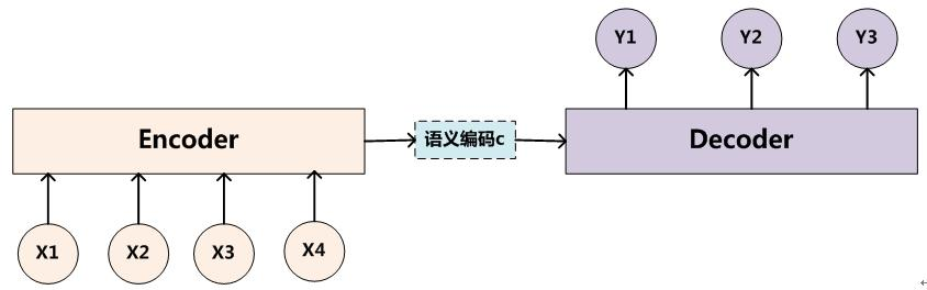
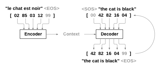
这次,我们仍然要自己搭建一个RNN,与第一篇和第二篇不同的是,这次是一个单词级别的RNN,是一个从序列到序列的模型,又叫做Seq2Seq(Sequence to Sequence)模型,常用到的结构是编码器-解码器结构(Encoder-Decoder)。在这个模型中,由两个循环神经网络同时工作,把一个序列转换成另一个序列。一个编码器神经网络会把输入的序列编码成一个上下文向量,然后把这个上下文向量输入解码器网络,解码器网络把它解码成一个新的序列。其结构如下图所示:

为了改进模型,我们还用到了一个注意力机制(Attention Mechanism),它使得解码器在每一步解码的时候,关注上下文向量中不同的范围。
2 基本原理
关于RNN的基础原理等,请见第一篇。
这里将简单介绍一下编码器-解码器以及注意力机制的原理。
序列
第一篇和第二篇都是字母级别的RNN,即对于输入 X = { x 1 , x 2 , … , x n } X=\{x_1,x_2,\ldots,x_n\} X={ x1,x2,…,xn}, X X X是一个单词, x i x_i xi是组成单词的字母,比如 X X X 是 “apple”,那么:
- x 1 x_1 x1:“a” 的one-hot编码
- x 2 x_2 x2:“p” 的one-hot编码
- x 3 x_3 x3:“p” 的one-hot编码
- x 4 x_4 x4:“l” 的one-hot编码
- x 5 x_5 x5:“e” 的one-hot编码
而在这一篇中是单词级别的RNN。
一句话可以看成是由词组成的序列。假设输入序列为 X = { x 1 , x 2 , … , x n } X=\{x_1,x_2,\ldots,x_n\} X={ x1,x2,…,xn}, x i x_i xi 是词典 V x V_x Vx 中的单词,输出序列为 Y = { y 1 , y 2 , … , y m } Y=\{y_1,y_2,\ldots,y_m\} Y={ y1,y2,…,ym}, y i y_i yi 是词典 V y V_y Vy 中的单词。
以机器翻译任务为例,假设输入一句法文 “vous etes trop maigre .” 那么输入序列就是:
- x 1 x_1 x1:“vous” 的one-hot编码
- x 2 x_2 x2:“etes” 的one-hot编码
- x 3 x_3 x3:“trop” 的one-hot编码
- x 4 x_4 x4:“maigre” 的one-hot编码
- x 5 x_5 x5:"." 的one-hot编码
输出一句英文 “ you re all alone .” 那么输出序列就是:
- y 1 y_1 y1:“you” 的one-hot编码
- y 2 y_2 y2:“re” 的one-hot编码
- y 3 y_3 y3:“all” 的one-hot编码
- y 4 y_4 y4:“alone” 的one-hot编码
- y 5 y_5 y5:"." 的one-hot编码
编码器-解码器
RNN的输入和输出关系可以分为几类:
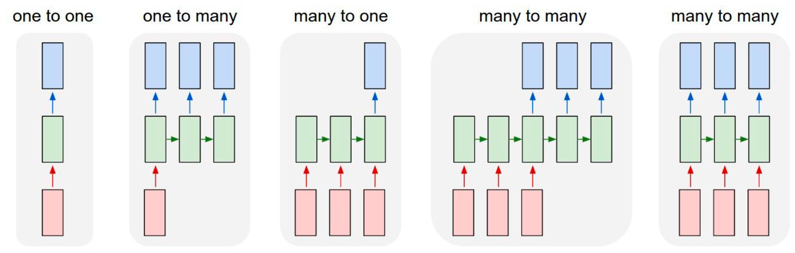
我们已经知道,一般的RNN,每一个输入都会对应产生一个输出:
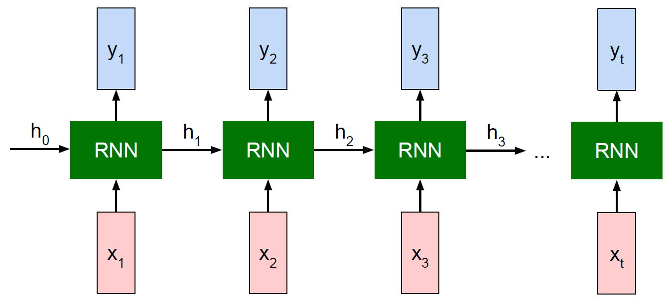
- 输入 x 1 x_{1} x1,输出 y 1 y_{1} y1
- 输入 x 2 x_{2} x2,输出 y 2 y_{2} y2
- ……
- 输入 x t x_{t} xt,输出 y t y_{t} yt
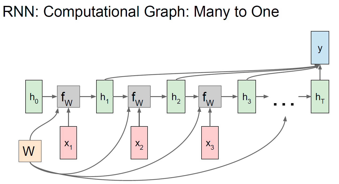
第一篇的RNN分类任务是典型的“多对一”的情况,我们用到的是模型最后一层的输出,通过softmax生成概率分布,从而进行分类
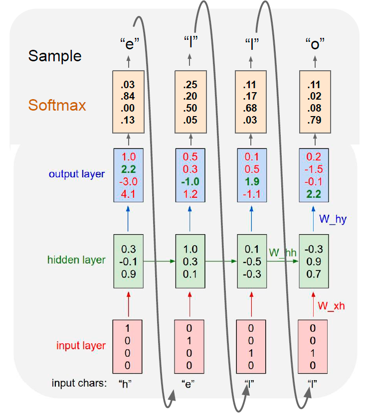
第二篇的RNN生成任务,本质上是“一对多”的情况,因为我们只输入了最开始的字母 x 1 x_1 x1,本来模型应该只输出 y 1 y_1 y1 就结束循环。RNN之后能够不断生成 y 2 y_2 y2、 y 3 y_3 y3、 y 4 y_4 y4……,是因为我们把前一步的输出 y t − 1 y_{t-1} yt−1 作为了下一步的输入 x t x_t xt,所以模型能够从“一对多”变成“多对多”。
回到我们的翻译任务,考虑我们自己做中英翻译,有时候,输入序列和输出序列是等长的,比如:“I have a pen”,可以翻译成“我有支笔”;有时候,输入序列和输出序列是不等长的,比如:"I have an apple ",翻译成“我有只苹果”,英文单词的数量是4,但是中文字的数量是5。
如何才能让输入序列和输出序列不等长?甚至输出序列比输入序列还长?有人想到了用两个RNN。一个RNN作为编码器,输入序列输入到RNN,然后它输出一个上下文向量(Context Vector) c c c,这个过程称为编码;另一个RNN作为解码器,把这个上下文向量 c c c 输入到RNN,它输出另一个输出序列,这个过程称为解码。如下图所示:
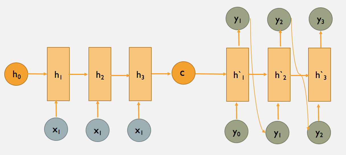
c c c 的左侧是编码器, c c c 的右侧是解码器。
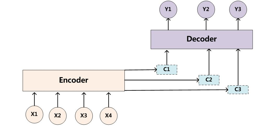
上图中的 c c c 只作为了解码器在第一步的输入,又有下面一种变体,即解码器的每一步都用到 c c c :
这相当于把“多对一”的RNN和“一对多”的RNN拼接在了一起,就可以完成我们的机器翻译任务。
注意力机制
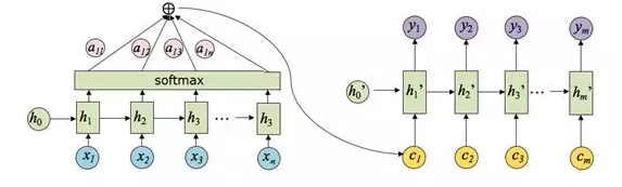
事实上,很难真正把输入序列的所有信息都压缩到一个向量 c c c 中,所以有人想到了用注意力机制,产生一个“注意力范围”。讲人话,就是解码器在每一步解码的时候,给编码器的隐藏层赋上不同的权重,用到不同的上下文向量 c t c_t ct。
普通的编码器-解码器如下图所示:
含有注意力机制的编码器-解码器如下图所示:
假设 h i h_i hi 是编码器第 i i i 步的隐藏层状态; h t ′ h'_t ht′ 是解码器第 t t t 步的隐藏层状态,上下文向量 c t c_t ct 的计算公式为:
c t = ∑ i = 1 ∣ Y ∣ α t i h i c_{t}=\sum_{i=1}^{|Y|} \alpha_{t i} h_{i} ct=i=1∑∣Y∣αtihi
α t i = exp ( e t i ) ∑ j = 1 ∣ Y ∣ exp ( e t j ) \alpha_{t i}= \frac{\exp \left(e_{t i}\right)}{\sum_{j=1}^{|Y|} \exp \left(e_{t j}\right)} αti=∑j=1∣Y∣exp(etj)exp(eti)
e t i = g ( h i , h t ′ ) e_{t i} =g\left(h_{i}, h'_{t}\right) eti=g(hi,ht′)
α t i \alpha_{t i} αti是注意力的权重,是 e t i e_{t i} eti 经过softmax函数后的值, e t i e_{t i} eti表示预测与目标的匹配打分函数。
c 1 c_1 c1 注意力权重的计算示例图如下图所示:
3 代码
数据预处理
首先,载入一些头文件。
from __future__ import unicode_literals, print_function, division
from io import open
import unicodedata
import string
import re
import random

import torch
import torch.nn as nn
from torch import optim
import torch.nn.functional as F

device = torch.device("cuda" if torch.cuda.is_available() else "cpu")
在Seq2Seq模型中,除了原有的词典外,还需要引入两个特殊符号,一个用于标记文本序列开始<SOS>(Start of String),一个用于标记文本序列结束<EOS>(End of String),它们的索引分别是0和1.
此外,对于英文和法文,都定义一个语言类 Lang,用于建立相应的词典。
和字母级别的RNN教程一样,每个单词都用一个 one-hot 向量来表示,即一堆0和一个1的向量,1所在的位置是这个单词的索引。与英文中只有26个字母相比,单词的数量要多得多,因此,对于英文和法文,我们都只选择一些数据来建立我们的词典。在英文数据上建立的词典 word2index 如下图所示:

索引为0的是 “<SOS>” 符号,索引为1的是 “<EOS>” 符号。
假设这里索引为2的是 “the” 这个单词,索引为3的是 “a” 这个单词,索引为4的是 “is” 这个单词,索引为5的是 “and” 这个单词,索引为6的是 “or” 这个单词……
那么 “and” 的one-hot向量即为:<0,0,0,0,0,1,0,…> (在5这个位置是1,其它位置都是0)
语言类 Lang 的定义如下:
word2index: word→index,是把单词映射为索引的词典index2word:index → word,是把索引映射为单词的词典word2count:统计出现过的单词总共出现的次数的词典n_words:词典中单词数量
SOS_token = 0
EOS_token = 1

class Lang:
    def __init__(self,name):
        self.name = name
        self.word2index = {
    } #把单词映射为索引的词典
        self.word2count = {
    } #统计出现过的单词总共出现的次数
        self.index2word = {
    0:"SOS", 1:"EOS"} #把索引映射为单词
        self.n_words = 2     #词典中单词数量

    def addSentence(self, sentence):
        # 把句子按空格分割,把句中每个单词都加入词典
        for word in sentence.split(' '):
            self.addWord(word)

    def addWord(self, word):
        # 如果单词之前没有出现过,就加入词典
        if word not in self.word2index:
            self.word2index[word] = self.n_words
            self.word2count[word] = 1
            self.index2word[self.n_words] = word
            self.n_words += 1
        # 如果单词之前已经出现过,就次数加1
        else:
            self.word2count[word] += 1
eng-fra.txt 是Unicode编码,把一些法文转化成普通的ASCII编码。此外,把句子中所有字母都转化成小写,并且移除一些不是字母的字符
# 把unicode编码转化成普通的ASCII编码
def unicodeToAscii(s):
    return ''.join(
        c for c in unicodedata.normalize('NFD', s)
        if unicodedata.category(c) != 'Mn'
    )

# 小写、移除一些不是字母的字符
def normalizeString(s):
    s = unicodeToAscii(s.lower().strip())
    s = re.sub(r"([.!?])", r" \1", s)
    s = re.sub(r"[^a-zA-Z.!?]+", r" ", s)
    return s
读入文件 eng-fra.txt。原来的文件是英译法,如果想法译英,可以把输入序列和输出序列交换一下,因此加入了一个 reverse 布尔值
def readLangs(lang1, lang2, reverse=False):
    print("Reading lines...")

    # 读入文件,并按回车分行,每一行都存储在lines中
    lines = open('data/%s-%s.txt' % (lang1, lang2),encoding='utf-8').read().strip().split('\n')

    # 每一行,用tab分割,前面的是英文,后面的是法文
    pairs = [[normalizeString(s) for s in line.split('\t')] for line in lines]

    # 如果reverse=True,就是法译英
    if reverse:
        pairs = [list(reversed(p)) for p in pairs]
        input_lang = Lang(lang2)
        output_lang = Lang(lang1)
    # 如果reverse=False,就是英译法
    else:
        input_lang = Lang(lang1)
        output_lang = Lang(lang2)

    return input_lang,output_lang,pairs
由于原来的文件中,样本句子有很多,为了加快训练,我们在本教程中,只用一些短小、简单的句子来创建训练集。我们去除了文件中长度大于 10 个单词(包含结尾标点符号)的句子,此外,我们只用以 “I am” 或 “He is” 等形式开头的句子。因为之前把 "i’m " 等缩写中的撇号(’)过滤掉了,所以这里是 "i m "。
MAX_LENGTH = 10 # 句子最大长度是10

# 过滤出一些长度不超过10,以下列前缀开头的句子作为训练集
eng_prefixes = (
    "i am ", "i m ",
    "he is", "he s ",
    "she is", "she s ",
    "you are", "you re ",
    "we are", "we re ",
    "they are", "they re"
)

def filterPair(p):
    return len(p[0].split(' ')) < MAX_LENGTH and\
      len(p[1].split(' ')) < MAX_LENGTH and\
      p[1].startswith(eng_prefixes)

def filterPairs(pairs):
    return [pair for pair in pairs if filterPair(pair)]
调用前面定义的函数,正式读入数据,并创建数据集:
- 读入文件,把文件分成行,然后每一行分成一个英-法句子对
- 把文本规则化,按长度和内容过滤出一些简单、短小的句子
- 从这些英-法句子对中创建词典
def prepareData(lang1, lang2, reverse=False):
    input_lang, output_lang, pairs = readLangs(lang1,lang2,reverse)
    print("Read %s sentence pairs" % len(pairs))
    pairs = filterPairs(pairs)
    print("Trimmed to %s sentence pairs" % len(pairs))
    print("Counting words...")
    for pair in pairs:
        input_lang.addSentence(pair[0]) # input_lang中为句子pair[0]创建词典
        output_lang.addSentence(pair[1]) # output_lang中为句子pair[1]创建词典
    print("Counted wrods:")
    print(input_lang.name,input_lang.n_words)
    print(output_lang.name,output_lang.n_words)
    return input_lang,output_lang,pairs

input_lang,output_lang,pairs=prepareData('eng','fra',True) #法译英
print(random.choice(pairs))
Out:
Reading lines...
Read 135842 sentence pairs
Trimmed to 10635 sentence pairs
Counting words...
Counted wrods:
fra 4370
eng 2824
['je suis une inconditionnelle de l opera allemand .', 'i m a fan of german opera .']
对于每一个英-法句子对,我们都需要一个输入的tensor(它是输入句子中的单词的索引)和一个目标的tensor(它是目标句子中的单词的索引)。在创建这些向量的时候,我们还需要给每个句子序列加入一个 “<EOS>” 符号:
# 创建句子的tensor
def indexesFromSentence(lang, sentence):
    return [lang.word2index[word] for word in sentence.split(' ')]

# 在句子的tensor中,加入EOS符号
def tensorFromSentence(lang, sentence):
    indexes = indexesFromSentence(lang,sentence)
    indexes.append(EOS_token)
    return torch.tensor(indexes, dtype = torch.long, device=device).view(-1,1)

# 创建句子对的tensor
def tensorsFromPair(pair):
    input_tensor = tensorFromSentence(input_lang,pair[0])
    target_tensor = tensorFromSentence(output_lang,pair[1])
    return (input_tensor, target_tensor)

sample_pairs = random.choice(pairs)
print(sample_pairs)
input_tensor, target_tensor = tensorsFromPair(sample_pairs)
print('input:',input_tensor)
print('target:',target_tensor)
Out:
['vous etes bonne .', 'you are good .']
input: tensor([[118],
        [214],
        [290],
        [  5],
        [  1]], device='cuda:0')
target: tensor([[129],
        [124],
        [ 44],
        [  4],
        [  1]], device='cuda:0')
模型
如前面所说,Seq2Seq模型中有两个RNN,一个是编码器,把输入序列编码成为一个向量 c c c,另一个是解码器,把向量 c c c解码成为一个输出序列。如下图所示:
编码器
Seq2Seq网络的编码器是一个RNN,在输入句子序列时,会为每一个单词输出一些值。对于每个输入的单词,编码器会输出一个向量和一个隐藏层状态,并将隐藏层状态用于下一个输入的单词。我们的编码器的示意图如下:
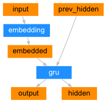
embedded 会将单词的one-hot向量变成词嵌入向量。
class EncoderRNN(nn.Module):
    def __init__(self,input_size,hidden_size):
        super(EncoderRNN, self).__init__()
        self.hidden_size = hidden_size
        self.embedding = nn.Embedding(input_size, hidden_size)
        self.gru = nn.GRU(hidden_size, hidden_size)

    def forward(self, input, hidden):
        embedded = self.embedding(input).view(1,1,-1)
        output, hidden = self.gru(embedded,hidden)
        return output,hidden

    def initHidden(self):
        return torch.zeros(1,1,self.hidden_size, device=device)
解码器
解码器是另一个RNN,它的输入是编码器输出的向量,然后解码器输出单词序列,从而进行机器翻译。
简单的解码器
在最简单的Seq2Seq模型中,解码器只用到编码器最后一层的输出。这最后一层的输出通常叫做上下文向量,因为它浓缩了输入序列的完整信息。这个上下文向量被用于初始化解码器的隐藏层状态。
在每一个解码的时候,会向解码器中输入一个符号和一个隐藏层状态,最开始的输入符号是 “<SOS>” 符号 ,标志着字符串的开始(Start-of-String),解码器的第一个隐藏层状态是上下文向量,即编码器最后一层的隐藏层状态。
普通的解码器的结构如下图所示:
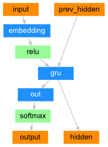
class DecoderRNN(nn.Module):
    def __init__(self, hidden_size, output_size):
        super(DecoderRNN, self).__init__()
        self.hidden_size = hidden_size
        self.embedding = nn.Embedding(output_size, hidden_size)
        self.gru = nn.GRU(hidden_size, hidden_size)
        self.out = nn.Linear(hidden_size, output_size)
        self.softmax = nn.LogSoftmax(dim=1)

    def forward(self, input, hidden):
        embedded = self.embedding(input).view(1,1,-1)
        embedded = F.relu(embedded)
        output, hidden = self.gru(embedded, hidden)
        output = self.softmax(self.out(output[0]))
        return output, hidden

    def initHidden(self):
        return torch.zeros(1,1,self.hidden_size, device=device)
你可以尝试用上面的解码器进行机器翻译,但是我们接下来会直接介绍一种更好的解码器——含注意力机制的解码器。
含注意力机制的解码器
如果光凭上下文向量把信息从编码器传递到解码器,那么它的负担太重——它要携带输入序列的完整信息。
注意力机制允许解码器在输出每一步的单词时,关注到编码器的输出的不同部分。首先,我们会计算一个注意力权重,然后,它们与编码器每一步输出的向量相乘,加权求和,得到一个向量。这个向量(代码中叫做 attn_applied )包含输入序列某一部分的信息,因此可以帮助解码器选择正确的输出单词。
由另一个前向传播的全连接层 attn 来计算注意力权重,它的输入是解码器的输入和隐藏层状态。因为在训练数据中,句子长度各不同,所以在训练这一层时,我们必须选择一个它能适用的最大句子长度。最大长度的句子将使用所有的注意力权重,而较短的句子只使用前几个。它的结构如下图所示:
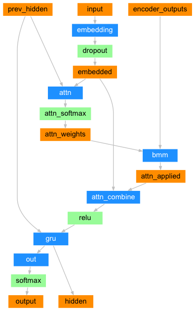
class AttnDecoderRNN(nn.Module):
    def __init__(self, hidden_size, output_size,
                dropout_p=0.1, max_length=MAX_LENGTH):
        super(AttnDecoderRNN, self).__init__()
        self.hidden_size = hidden_size
        self.output_size = output_size # 目标语言的单词数量
        self.dropout_p = dropout_p
        self.max_length = max_length

        self.embedding = nn.Embedding(self.output_size, self.hidden_size)
        self.attn = nn.Linear(self.hidden_size * 2,self.max_length)
        self.attn_combine = nn.Linear(self.hidden_size * 2,self.hidden_size)
        self.dropout = nn.Dropout(self.dropout_p)
        self.gru = nn.GRU(self.hidden_size, self.hidden_size)
        self.out = nn.Linear(self.hidden_size, self.output_size)

    def forward(self, input, hidden, encoder_outputs):
        # input是编码器的上一步输出 或者 真实的前一个单词
        embedded = self.embedding(input).view(1,1,-1)
        embedded = self.dropout(embedded)

        # 计算注意力权重
        attn_weights = F.softmax(
            self.attn(torch.cat((embedded[0],hidden[0]),1)),dim=1)

        # torch.bmm(a,b):计算两个tensor的Hadamard乘积,
        # tensor a 的大小为(b,h1,w),
        # tensor b 的大小为(b,w,h2)
        attn_applied = torch.bmm(attn_weights.unsqueeze(0), # 1, 1, max_length
                    encoder_outputs.unsqueeze(0)) # 1, max_length, hidden_size

        # 输出的attn_applied 大小为 (1, 1, hidden_size)
        # embedded: (1, 1, hidden_size)
        output = torch.cat((embedded[0], attn_applied[0]),1)
        output = self.attn_combine(output).unsqueeze(0)

        output = F.relu(output)
        output, hidden = self.gru(output,hidden)

        output = F.log_softmax(self.out(output[0]),dim=1)
        return output, hidden, attn_weights

    def initHidden(self):
        return torch.zeros(1,1,self.hidden_size,device=device)
训练
为了训练,我们先把输入序列通过编码器,然后用 encoder_outputs 记录编码器每一步的输出和最后一步的隐藏层状态。然后,我们给解码器输入 “<SOS>” 符号作为第一个输入,然后把编码器最后一步的隐藏层状态作为解码器第一步的隐藏层状态。
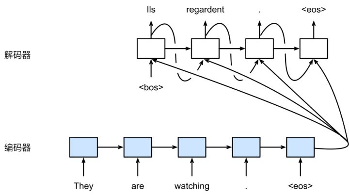
“Teacher forcing”是一个加速RNN收敛的技巧。如下图所示:
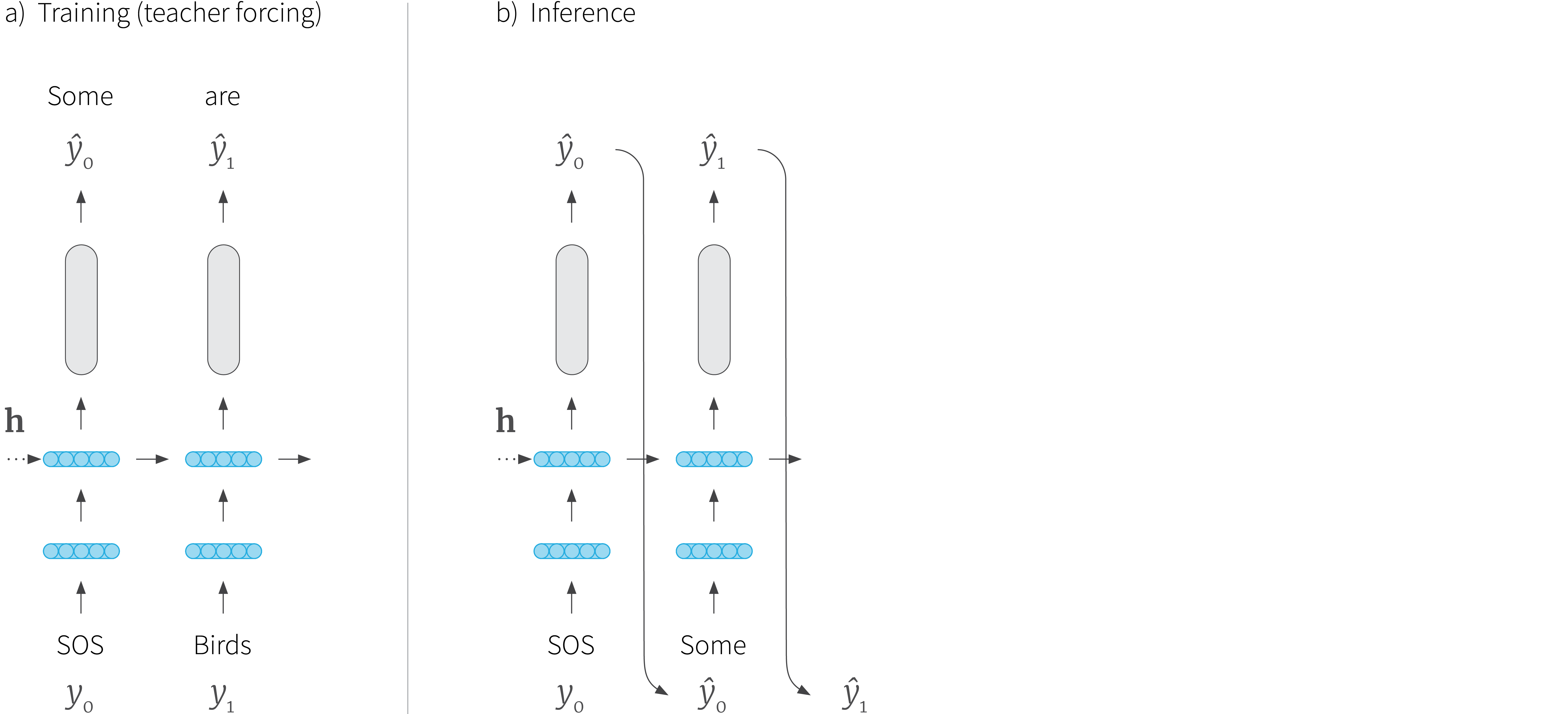
我们原本是拿RNN上一步的预测值 y t − 1 y_{t-1} yt−1 作为当前的输入 x t x_t xt,这个方法叫做自回归(Autoregressive)。但是,RNN刚开始训练时,预测效果不好,如果一味任凭RNN自己训练,一旦它某一步预测错误,之后的预测就会偏离目标值越来越远;而“Teacher forcing”中用真实的目标单词 y t − 1 ∗ y^*_{t-1} yt−1∗ 作为当前的输入 x t x_t xt,帮助模型学习与快速收敛。不过,“Teacher forcing”也存在着问题:当我们用训练好的模型进行测试时,它可能会表现得不稳定。
因此,我们需要限制“Teacher forcing”和自回归的比例,用到了teacher_forcing_ratio,即有 p p p 的概率,选择“Teacher forcing”,输入真值 y t − 1 ∗ y^*_{t-1} yt−1∗ ,有 1 − p 1-p 1−p 的概率选择自回归,输入预测值 y t − 1 y_{t-1} yt−1。
teacher_forcing_ratio = 0.5

def train(input_tensor, target_tensor, encoder, decoder,
      encoder_optimizer, decoder_optimizer, criterion, max_length=MAX_LENGTH):
    encoder_hidden = encoder.initHidden()

    encoder_optimizer.zero_grad()
    decoder_optimizer.zero_grad()

    input_length = input_tensor.size(0)  # 源语言句子长度
    target_length = target_tensor.size(0) # 目标语言句子长度

    encoder_outputs = torch.zeros(max_length,encoder.hidden_size,device=device)

    loss = 0

    for ei in range(input_length):
        encoder_output, encoder_hidden = encoder(
            input_tensor[ei],encoder_hidden)
        encoder_outputs[ei] = encoder_output[0,0]  # 保存encoder每一步的隐藏层状态

    decoder_input = torch.tensor([[SOS_token]],device=device) # decoder的第一个输入是SOS

    decoder_hidden = encoder_hidden # encoder最后一步隐藏层状态

    use_teacher_forcing = True if random.random()<teacher_forcing_ratio else False

    if use_teacher_forcing:
    # 强制输入target的input
        for di in range(target_length):
            decoder_output, decoder_hidden, decoder_attention = decoder(
              decoder_input, decoder_hidden, encoder_outputs)
            loss += criterion(decoder_output, target_tensor[di])
            decoder_input = target_tensor[di]

    else:
    # 输入预测的input
        for di in range(target_length):
            decoder_output, decoder_hidden, decoder_attention = decoder(
              decoder_input, decoder_hidden, encoder_outputs)
            topv,topi = decoder_output.topk(1)
            decoder_input = topi.squeeze().detach()

            loss += criterion(decoder_output, target_tensor[di])

            if decoder_input.item() == EOS_token: break

    loss.backward()

    encoder_optimizer.step()
    decoder_optimizer.step()

    return loss.item()/target_length
与前两篇相同,让我们在训练时记录已训练的时间、剩余训练时间、损失等信息。
import time
import math

def asMinutes(s):
    m = math.floor(s / 60)
    s -= m * 60
    return '%dm %ds' % (m, s)

def timeSince(since, percent):
    now = time.time()
    s = now - since
    es = s / (percent)
    rs = es - s
    return '%s (- %s)' % (asMinutes(s), asMinutes(rs))
整个训练过程如下:
- 开始一个计时器
- 初始化优化器 optimizers 和损失函数 criterion
- 创建训练的样本对
- 在数组中记录损失,用于之后画图
%matplotlib inline
import matplotlib
import matplotlib.pyplot as plt
import matplotlib.ticker as ticker
import numpy as np
def showPlot(points):
plt.figure()
fig, ax = plt.subplots()
# this locator puts ticks at regular intervals
loc = ticker.MultipleLocator(base=0.2)
ax.yaxis.set_major_locator(loc)
plt.plot(points)
def trainIters(encoder, decoder, n_iters, print_every=1000,
plot_every=100,learning_rate = 0.01):
start = time.time()
plot_losses = []
print_loss_total = 0
plot_loss_total = 0
encoder_optimizer = optim.SGD(encoder.parameters(),lr=learning_rate)
decoder_optimizer = optim.SGD(decoder.parameters(),lr=learning_rate)
training_pairs = [tensorsFromPair(random.choice(pairs)) for i in range(n_iters)]
criterion = nn.NLLLoss()
for iter in range(1,n_iters+1):
training_pair = training_pairs[iter-1]
input_tensor = training_pair[0]
target_tensor = training_pair[1]
loss = train(input_tensor, target_tensor,encoder,
decoder, encoder_optimizer, decoder_optimizer,criterion)
print_loss_total += loss
plot_loss_total += loss
if iter % print_every ==0:
print_loss_avg = print_loss_total/print_every
print_loss_total = 0
print("%s (%d %d%%) %.4f"%(timeSince(start,iter/n_iters),
iter, iter / n_iters*100, print_loss_avg))
if iter % plot_every == 0:
plot_loss_avg = plot_loss_total / plot_every
plot_losses.append(plot_loss_avg)
plot_loss_total =0
showPlot(plot_losses)
hidden_size = 256
encoder1 = EncoderRNN(input_lang.n_words, hidden_size).to(device)
attn_decoder1 = AttnDecoderRNN(hidden_size, output_lang.n_words, dropout_p=0.1).to(device)
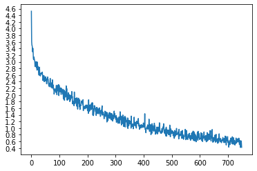
trainIters(encoder1,attn_decoder1,75000,print_every=5000)
运行了71分钟,终于训练完了……
Out:
5m 0s (- 70m 2s) (5000 6%) 2.8654
9m 35s (- 62m 22s) (10000 13%) 2.2857
14m 21s (- 57m 27s) (15000 20%) 2.0029
19m 7s (- 52m 36s) (20000 26%) 1.7256
23m 48s (- 47m 37s) (25000 33%) 1.5591
28m 26s (- 42m 39s) (30000 40%) 1.3824
33m 15s (- 38m 1s) (35000 46%) 1.2276
38m 3s (- 33m 18s) (40000 53%) 1.1112
42m 51s (- 28m 34s) (45000 60%) 0.9992
47m 40s (- 23m 50s) (50000 66%) 0.9228
52m 27s (- 19m 4s) (55000 73%) 0.8154
57m 16s (- 14m 19s) (60000 80%) 0.7489
62m 5s (- 9m 33s) (65000 86%) 0.7264
66m 59s (- 4m 47s) (70000 93%) 0.6505
71m 44s (- 0m 0s) (75000 100%) 0.5862
测试
测试过程和训练过程相同,但是没有真值,因此我们将解码器上一步的预测值作为它当前的输入。它每预测一个词,我们就把这个词加入输出的字符串中,如果它预测到了“<EOS>” 符号,我们就停止RNN的循环。另外,我们还要保存解码器的注意力输出,之后用于画图。
def evaluate(encoder, decoder, sentence, max_length =MAX_LENGTH):
    with torch.no_grad():
        input_tensor = tensorFromSentence(input_lang,sentence)
        input_length = input_tensor.size()[0]
        encoder_hidden = encoder.initHidden()

        encoder_outputs = torch.zeros(max_length,encoder.hidden_size,device=device)

        for ei in range(input_length):
            encoder_output, encoder_hidden = encoder(input_tensor[ei],encoder_hidden)
            encoder_outputs[ei] += encoder_output[0,0]

        decoder_input = torch.tensor([[SOS_token]],device=device)

        decoder_hidden=encoder_hidden

        decoded_words = []
        decoder_attentions = torch.zeros(max_length, max_length)

        for di in range(max_length):
            decoder_output, decoder_hidden,decoder_attention = decoder(decoder_input,decoder_hidden,encoder_outputs)
            decoder_attentions[di] = decoder_attention.data
            topv, topi = decoder_output.data.topk(1)
            if topi.item() == EOS_token:
                decoded_words.append('<EOS>')
                break
            else:
                decoded_words.append(output_lang.index2word[topi.item()])

            decoder_input = topi.squeeze().detach()

        return decoded_words, decoder_attentions[:di+1]
测试10个样例
def evaluateRandomly(encoder,decoder,n=10):
    for i in range(n):
        pair = random.choice(pairs)
        print('>', pair[0])
        print('=', pair[1])
        output_words, attentions = evaluate(encoder, decoder, pair[0])
        output_sentence = ' '.join(output_words)
        print('<', output_sentence)
        print('')

evaluateRandomly(encoder1, attn_decoder1)
Out:
> j ai faim et soif .
= i m hungry and thirsty .
< i m hungry and thirsty . <EOS>

> j ai les glandes .
= i m really angry .
< i m really angry . <EOS>

> je suis desolee si je vous ai effrayees .
= i m sorry if i frightened you .
< i m sorry if i frightened you . <EOS>

> vous n etes pas tres bons .
= you re not very good .
< you re not very good . <EOS>

> je ne suis pas quelqu un de patient .
= i m not a patient person .
< i m not a drunk person . <EOS>

> je te le demande en tant qu ami .
= i m asking you as a friend .
< i m asking you as a friend . <EOS>

> vous etes paranoiaques .
= you re being paranoid .
< you re clever . <EOS>

> vous etes plus intelligents que moi .
= you re smarter than me .
< you re smarter than me . <EOS>

> elle fait un regime pour perdre du poids .
= she is on a diet to lose weight .
< she s on weight for lose weight . <EOS>

> j ai la schcoumoune .
= i m unlucky .
< i m learning . <EOS>
画图
我们画出在翻译某句句子时的注意力权重 attentions
output_words, attentions = evaluate(
    encoder1, attn_decoder1, "je suis trop froid .")
plt.matshow(attentions.cpu().numpy())
Out:

为了更直观,我们加上坐标轴和标签:
def showAttention(input_sentence, output_words, attentions):
    # Set up figure with colorbar
    fig = plt.figure()
    ax = fig.add_subplot(111)
    cax = ax.matshow(attentions.numpy(), cmap='bone')
    fig.colorbar(cax)

    # Set up axes
    ax.set_xticklabels([''] + input_sentence.split(' ') +
                      ['<EOS>'], rotation=90)
    ax.set_yticklabels([''] + output_words)

    # Show label at every tick
    ax.xaxis.set_major_locator(ticker.MultipleLocator(1))
    ax.yaxis.set_major_locator(ticker.MultipleLocator(1))

    plt.show()

def evaluateAndShowAttention(input_sentence):
    output_words, attentions = evaluate(
      encoder1, attn_decoder1, input_sentence)
    print('input = ',input_sentence)
    print('output = ',' '.join(output_words))
    showAttention(input_sentence, output_words, attentions)

evaluateAndShowAttention("elle a cinq ans de moins que moi .")

evaluateAndShowAttention("elle est trop petit .")

evaluateAndShowAttention("je ne crains pas de mourir .")

evaluateAndShowAttention("c est un jeune directeur plein de talent .")
Out:
input =  elle a cinq ans de moins que moi .
output =  she s five years younger than i am . <EOS>

input =  elle est trop petit .
output =  she s too short . <EOS>

input =  je ne crains pas de mourir .
output =  i m not scared of dying . <EOS>

input =  c est un jeune directeur plein de talent .
output =  he s a very young . <EOS>

至此,本教程已结束。你可以尝试更多练习:
-
尝试不同的训练集:
- 另一种语言对的翻译
- 人类语言 → 机器语言(比如 IOT 命令)
- 对话 → 回复
- 问题 → 答案
-
把词嵌入层换成预训练的词嵌入模型,比如 word2vec 或者 GloVe
-
用更多层、更多隐藏层单元、更多训练数据,比较训练时间和结果
-
如果你用的翻译数据集中有两个相同的短语,比如
I am test \t I am test,你可以尝试自编码器
参考资料
智能推荐
oracle 12c 集群安装后的检查_12c查看crs状态-程序员宅基地
文章浏览阅读1.6k次。安装配置gi、安装数据库软件、dbca建库见下:http://blog.csdn.net/kadwf123/article/details/784299611、检查集群节点及状态:[root@rac2 ~]# olsnodes -srac1 Activerac2 Activerac3 Activerac4 Active[root@rac2 ~]_12c查看crs状态
解决jupyter notebook无法找到虚拟环境的问题_jupyter没有pytorch环境-程序员宅基地
文章浏览阅读1.3w次,点赞45次,收藏99次。我个人用的是anaconda3的一个python集成环境,自带jupyter notebook,但在我打开jupyter notebook界面后,却找不到对应的虚拟环境,原来是jupyter notebook只是通用于下载anaconda时自带的环境,其他环境要想使用必须手动下载一些库:1.首先进入到自己创建的虚拟环境(pytorch是虚拟环境的名字)activate pytorch2.在该环境下下载这个库conda install ipykernelconda install nb__jupyter没有pytorch环境
国内安装scoop的保姆教程_scoop-cn-程序员宅基地
文章浏览阅读5.2k次,点赞19次,收藏28次。选择scoop纯属意外,也是无奈,因为电脑用户被锁了管理员权限,所有exe安装程序都无法安装,只可以用绿色软件,最后被我发现scoop,省去了到处下载XXX绿色版的烦恼,当然scoop里需要管理员权限的软件也跟我无缘了(譬如everything)。推荐添加dorado这个bucket镜像,里面很多中文软件,但是部分国外的软件下载地址在github,可能无法下载。以上两个是官方bucket的国内镜像,所有软件建议优先从这里下载。上面可以看到很多bucket以及软件数。如果官网登陆不了可以试一下以下方式。_scoop-cn
Element ui colorpicker在Vue中的使用_vue el-color-picker-程序员宅基地
文章浏览阅读4.5k次,点赞2次,收藏3次。首先要有一个color-picker组件 <el-color-picker v-model="headcolor"></el-color-picker>在data里面data() { return {headcolor: ’ #278add ’ //这里可以选择一个默认的颜色} }然后在你想要改变颜色的地方用v-bind绑定就好了,例如:这里的:sty..._vue el-color-picker
迅为iTOP-4412精英版之烧写内核移植后的镜像_exynos 4412 刷机-程序员宅基地
文章浏览阅读640次。基于芯片日益增长的问题,所以内核开发者们引入了新的方法,就是在内核中只保留函数,而数据则不包含,由用户(应用程序员)自己把数据按照规定的格式编写,并放在约定的地方,为了不占用过多的内存,还要求数据以根精简的方式编写。boot启动时,传参给内核,告诉内核设备树文件和kernel的位置,内核启动时根据地址去找到设备树文件,再利用专用的编译器去反编译dtb文件,将dtb还原成数据结构,以供驱动的函数去调用。firmware是三星的一个固件的设备信息,因为找不到固件,所以内核启动不成功。_exynos 4412 刷机
Linux系统配置jdk_linux配置jdk-程序员宅基地
文章浏览阅读2w次,点赞24次,收藏42次。Linux系统配置jdkLinux学习教程,Linux入门教程(超详细)_linux配置jdk
随便推点
matlab(4):特殊符号的输入_matlab微米怎么输入-程序员宅基地
文章浏览阅读3.3k次,点赞5次,收藏19次。xlabel('\delta');ylabel('AUC');具体符号的对照表参照下图:_matlab微米怎么输入
C语言程序设计-文件(打开与关闭、顺序、二进制读写)-程序员宅基地
文章浏览阅读119次。顺序读写指的是按照文件中数据的顺序进行读取或写入。对于文本文件,可以使用fgets、fputs、fscanf、fprintf等函数进行顺序读写。在C语言中,对文件的操作通常涉及文件的打开、读写以及关闭。文件的打开使用fopen函数,而关闭则使用fclose函数。在C语言中,可以使用fread和fwrite函数进行二进制读写。 Biaoge 于2024-03-09 23:51发布 阅读量:7 ️文章类型:【 C语言程序设计 】在C语言中,用于打开文件的函数是____,用于关闭文件的函数是____。
Touchdesigner自学笔记之三_touchdesigner怎么让一个模型跟着鼠标移动-程序员宅基地
文章浏览阅读3.4k次,点赞2次,收藏13次。跟随鼠标移动的粒子以grid(SOP)为partical(SOP)的资源模板,调整后连接【Geo组合+point spirit(MAT)】,在连接【feedback组合】适当调整。影响粒子动态的节点【metaball(SOP)+force(SOP)】添加mouse in(CHOP)鼠标位置到metaball的坐标,实现鼠标影响。..._touchdesigner怎么让一个模型跟着鼠标移动
【附源码】基于java的校园停车场管理系统的设计与实现61m0e9计算机毕设SSM_基于java技术的停车场管理系统实现与设计-程序员宅基地
文章浏览阅读178次。项目运行环境配置:Jdk1.8 + Tomcat7.0 + Mysql + HBuilderX(Webstorm也行)+ Eclispe(IntelliJ IDEA,Eclispe,MyEclispe,Sts都支持)。项目技术:Springboot + mybatis + Maven +mysql5.7或8.0+html+css+js等等组成,B/S模式 + Maven管理等等。环境需要1.运行环境:最好是java jdk 1.8,我们在这个平台上运行的。其他版本理论上也可以。_基于java技术的停车场管理系统实现与设计
Android系统播放器MediaPlayer源码分析_android多媒体播放源码分析 时序图-程序员宅基地
文章浏览阅读3.5k次。前言对于MediaPlayer播放器的源码分析内容相对来说比较多,会从Java-&amp;gt;Jni-&amp;gt;C/C++慢慢分析,后面会慢慢更新。另外,博客只作为自己学习记录的一种方式,对于其他的不过多的评论。MediaPlayerDemopublic class MainActivity extends AppCompatActivity implements SurfaceHolder.Cal..._android多媒体播放源码分析 时序图
java 数据结构与算法 ——快速排序法-程序员宅基地
文章浏览阅读2.4k次,点赞41次,收藏13次。java 数据结构与算法 ——快速排序法_快速排序法