目录

一、说明

二、函数和参数详解

2.1 scatter函数原型

2.2 参数详解

2.3 其中散点的形状参数marker如下：

2.4 其中颜色参数c如下:

三、画图示例

3.1 关于坐标x，y和s，c

3.2 多元高斯的情况

3.3  绘制例子

3.4 绘图例3

3.5  同心绘制

3.6 有标签绘制

3.7 直线划分

3.8 曲线划分

---

一、说明

       关于matplotlib的scatter函数有许多活动参数，如果不专门注解，是无法掌握精髓的，本文专门针对scatter的参数和调用说起，并配有若干案例。

二、函数和参数详解

2.1 scatter函数原型

matplotlib.pyplot.scatter(x, y, s=None, c=None, marker=None, cmap=None, norm=None, vmin=None, vmax=None, alpha=None, linewidths=None, *, edgecolors=None, plotnonfinite=False, data=None, **kwargs)

2.2 参数详解

属性	参数	意义
坐标	x，y	输入点列的数组，长度都是size
点大小	s	点的直径数组，默认直径20，长度最大size
点颜色	c	点的颜色，默认蓝色 'b'，也可以是个 RGB 或 RGBA 二维行数组。
点形状	marker	点的样式，默认小圆圈 'o'。
调色板	cmap	Colormap，默认 None，标量或者是一个 colormap 的名字，只有 c 是一个浮点数数组时才使用。如果没有申明就是 image.cmap。
亮度（1）	norm	Normalize，默认 None，数据亮度在 0-1 之间，只有 c 是一个浮点数的数组的时才使用。
亮度（2）	vmin，vmax	亮度设置，在 norm 参数存在时会忽略。
透明度	alpha	透明度设置，0-1 之间，默认 None，即不透明
线	linewidths	标记点的长度
颜色	edgecolors	颜色或颜色序列，默认为 'face'，可选值有 'face', 'none', None。
	plotnonfinite	布尔值，设置是否使用非限定的 c ( inf, -inf 或 nan) 绘制点。
	**kwargs	其他参数。

2.3 其中散点的形状参数marker如下：

2.4 其中颜色参数c如下:

三、画图示例

3.1 关于坐标x，y和s，c

import numpy as np
import matplotlib.pyplot as plt

# Fixing random state for reproducibility
np.random.seed(19680801)


N = 50
x = np.random.rand(N)
y = np.random.rand(N)
colors = np.random.rand(N)          # 颜色可以随机
area = (30 * np.random.rand(N))**2  # 点的宽度30，半径15

plt.scatter(x, y, s=area, c=colors, alpha=0.5)  
plt.show()

        注意：以上核心语句是：

plt.scatter(x, y, s=area, c=colors, alpha=0.5, marker=",")

        其中：x，y，s，c维度一样就能成。

3.2 多元高斯的情况

​
import numpy as np
import matplotlib.pyplot as plt


fig=plt.figure(figsize=(8,6))
#Generating a Gaussion dataset:
#creating random vectors from the multivariate normal distribution
#given mean and covariance
mu_vec1=np.array([0,0])
cov_mat1=np.array([[1,0],[0,1]])
X=np.random.multivariate_normal(mu_vec1,cov_mat1,500)
R=X**2
R_sum=R.sum(axis=1)
plt.scatter(X[:,0],X[:,1],color='green',marker='o', =32.*R_sum,edgecolor='black',alpha=0.5)

plt.show()

​

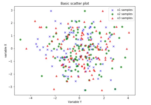
3.3  绘制例子

from matplotlib import pyplot as plt
import numpy as np
# Generating a Gaussion dTset:
#Creating random vectors from the multivaritate normal distribution
#givem mean and covariance

mu_vecl = np.array([0, 0])
cov_matl = np.array([[2,0],[0,2]])

x1_samples = np.random.multivariate_normal(mu_vecl, cov_matl,100)
x2_samples = np.random.multivariate_normal(mu_vecl+0.2, cov_matl +0.2, 100)
x3_samples = np.random.multivariate_normal(mu_vecl+0.4, cov_matl +0.4, 100)

plt.figure(figsize = (8, 6))

plt.scatter(x1_samples[:,0], x1_samples[:, 1], marker='x',
           color = 'blue', alpha=0.7, label = 'x1 samples')
plt.scatter(x2_samples[:,0], x1_samples[:,1], marker='o',
           color ='green', alpha=0.7, label = 'x2 samples')
plt.scatter(x3_samples[:,0], x1_samples[:,1], marker='^',
           color ='red', alpha=0.7, label = 'x3 samples')
plt.title('Basic scatter plot')
plt.ylabel('variable X')
plt.xlabel('Variable Y')
plt.legend(loc = 'upper right')

plt.show()


    import matplotlib.pyplot as plt
    
    fig,ax = plt.subplots()
    
    ax.plot([0],[0], marker="o",  markersize=10)
    ax.plot([0.07,0.93],[0,0],    linewidth=10)
    ax.scatter([1],[0],           s=100)
    
    ax.plot([0],[1], marker="o",  markersize=22)
    ax.plot([0.14,0.86],[1,1],    linewidth=22)
    ax.scatter([1],[1],           s=22**2)
    
    plt.show()



![image.png](http://upload-images.jianshu.io/upload_images/8730384-8d27a5015b37ee97.png?imageMogr2/auto-orient/strip%7CimageView2/2/w/1240)

    import matplotlib.pyplot as plt
    
    for dpi in [72,100,144]:
    
        fig,ax = plt.subplots(figsize=(1.5,2), dpi=dpi)
        ax.set_title("fig.dpi={}".format(dpi))
    
        ax.set_ylim(-3,3)
        ax.set_xlim(-2,2)
    
        ax.scatter([0],[1], s=10**2, 
                   marker="s", linewidth=0, label="100 points^2")
        ax.scatter([1],[1], s=(10*72./fig.dpi)**2, 
                   marker="s", linewidth=0, label="100 pixels^2")
    
        ax.legend(loc=8,framealpha=1, fontsize=8)
    
        fig.savefig("fig{}.png".format(dpi), bbox_inches="tight")
    
    plt.show() 

3.4 绘图例3

import matplotlib.pyplot as plt

for dpi in [72,100,144]:

    fig,ax = plt.subplots(figsize=(1.5,2), dpi=dpi)
    ax.set_title("fig.dpi={}".format(dpi))

    ax.set_ylim(-3,3)
    ax.set_xlim(-2,2)

    ax.scatter([0],[1], s=10**2, 
               marker="s", linewidth=0, label="100 points^2")
    ax.scatter([1],[1], s=(10*72./fig.dpi)**2, 
               marker="s", linewidth=0, label="100 pixels^2")

    ax.legend(loc=8,framealpha=1, fontsize=8)

    fig.savefig("fig{}.png".format(dpi), bbox_inches="tight")

plt.show() 

3.5  同心绘制

plt.scatter(2, 1, s=4000, c='r')
plt.scatter(2, 1, s=1000 ,c='b')
plt.scatter(2, 1, s=10, c='g')

3.6 有标签绘制

import matplotlib.pyplot as plt

x_coords = [0.13, 0.22, 0.39, 0.59, 0.68, 0.74,0.93]
y_coords = [0.75, 0.34, 0.44, 0.52, 0.80, 0.25,0.55]

fig = plt.figure(figsize = (8,5))

plt.scatter(x_coords, y_coords, marker = 's', s = 50)
for x, y in zip(x_coords, y_coords):
    plt.annotate('(%s,%s)'%(x,y), xy=(x,y),xytext = (0, -10), textcoords = 'offset points',ha = 'center', va = 'top')
plt.xlim([0,1])
plt.ylim([0,1])
plt.show()

3.7 直线划分

# 2-category classfication with random 2D-sample data
# from a multivariate normal distribution

import numpy as np
from matplotlib import pyplot as plt

def decision_boundary(x_1):
    """Calculates the x_2 value for plotting the decision boundary."""
#    return 4 - np.sqrt(-x_1**2 + 4*x_1 + 6 + np.log(16))
    return -x_1 + 1

# Generating a gaussion dataset:
# creating random vectors from the multivariate normal distribution
# given mean and covariance

mu_vec1 = np.array([0,0])
cov_mat1 = np.array([[2,0],[0,2]])
x1_samples = np.random.multivariate_normal(mu_vec1, cov_mat1,100)
mu_vec1 = mu_vec1.reshape(1,2).T # TO 1-COL VECTOR

mu_vec2 = np.array([1,2])
cov_mat2 = np.array([[1,0],[0,1]])
x2_samples = np.random.multivariate_normal(mu_vec2, cov_mat2, 100)
mu_vec2 = mu_vec2.reshape(1,2).T # to 2-col vector

# Main scatter plot and plot annotation

f, ax = plt.subplots(figsize = (7, 7))
ax.scatter(x1_samples[:, 0], x1_samples[:,1], marker = 'o',color = 'green', s=40)
ax.scatter(x2_samples[:, 0], x2_samples[:,1], marker = '^',color = 'blue', s =40)
plt.legend(['Class1 (w1)', 'Class2 (w2)'], loc = 'upper right')
plt.title('Densities of 2 classes with 25 bivariate random patterns each')
plt.ylabel('x2')
plt.xlabel('x1')
ftext = 'p(x|w1) -N(mu1=(0,0)^t, cov1 = I)\np.(x|w2) -N(mu2 = (1, 1)^t), cov2 =I'
plt.figtext(.15,.8, ftext, fontsize = 11, ha ='left')

#Adding decision boundary to plot

x_1 = np.arange(-5, 5, 0.1)
bound = decision_boundary(x_1)
plt.plot(x_1, bound, 'r--', lw = 3)

x_vec = np.linspace(*ax.get_xlim())
x_1 = np.arange(0, 100, 0.05)

plt.show()

3.8 曲线划分

# 2-category classfication with random 2D-sample data
# from a multivariate normal distribution

import numpy as np
from matplotlib import pyplot as plt

def decision_boundary(x_1):
    """Calculates the x_2 value for plotting the decision boundary."""
    return 4 - np.sqrt(-x_1**2 + 4*x_1 + 6 + np.log(16))

# Generating a gaussion dataset:
# creating random vectors from the multivariate normal distribution
# given mean and covariance

mu_vec1 = np.array([0,0])
cov_mat1 = np.array([[2,0],[0,2]])
x1_samples = np.random.multivariate_normal(mu_vec1, cov_mat1,100)
mu_vec1 = mu_vec1.reshape(1,2).T # TO 1-COL VECTOR

mu_vec2 = np.array([1,2])
cov_mat2 = np.array([[1,0],[0,1]])
x2_samples = np.random.multivariate_normal(mu_vec2, cov_mat2, 100)
mu_vec2 = mu_vec2.reshape(1,2).T # to 2-col vector

# Main scatter plot and plot annotation

f, ax = plt.subplots(figsize = (7, 7))
ax.scatter(x1_samples[:, 0], x1_samples[:,1], marker = 'o',color = 'green', s=40)
ax.scatter(x2_samples[:, 0], x2_samples[:,1], marker = '^',color = 'blue', s =40)
plt.legend(['Class1 (w1)', 'Class2 (w2)'], loc = 'upper right')
plt.title('Densities of 2 classes with 25 bivariate random patterns each')
plt.ylabel('x2')
plt.xlabel('x1')
ftext = 'p(x|w1) -N(mu1=(0,0)^t, cov1 = I)\np.(x|w2) -N(mu2 = (1, 1)^t), cov2 =I'
plt.figtext(.15,.8, ftext, fontsize = 11, ha ='left')

#Adding decision boundary to plot

x_1 = np.arange(-5, 5, 0.1)
bound = decision_boundary(x_1)
plt.plot(x_1, bound, 'r--', lw = 3)

x_vec = np.linspace(*ax.get_xlim())
x_1 = np.arange(0, 100, 0.05)

plt.show()