TensorFlow图像分类:如何构建分类器-程序员宅基地
导言
图像分类对于我们来说是一件非常容易的事情,但是对于一台机器来说,在人工智能和深度学习广泛使用之前,这是一项艰巨的任务。自动驾驶汽车能够实时检测物体并采取相应必要的行动,并且由于TensorFlow图像分类,大部分都可以实现。
在本文中,将你共同学习以下内容:
什么是TensorFlow?
什么是图像分类?
TensorFlow图像分类:Fashion-MNIST
CIFAR 10:CNN
什么是TensorFlow?
TensorFlow是Google的开源机器学习框架,用于跨越一些列任务进行数据流编程。图中的节点表示数学运算,而图表边表示在它们之间传递的多维数据阵列。
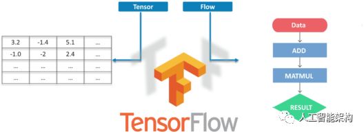
Tensors是多维数组,是二维表到具有更高维度的数据的扩展。TensorFlow的许多功能使其适合深度学习,它的核心开源库可以帮助大家开发和训练ML模型。
什么是图像分类?
图像分类的目的是将数字图像中的所有像素分类为若干类或主题之一。然后,该分类数据可用于显示图像中的物体是否存在与以上分类或主题。

根据分类过程中的交互,有两种类型的分类:
监督
无监督
所以,我们直接通过两个例子学习TensorFlow图像分类。
TensorFlow图像分类:Fashion-MNIST
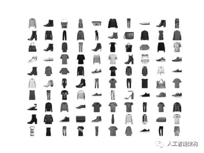
Fashion-MNIST数据集
在这里,我们将使用Fashion MNIST Dataset,它包含10个类别中的70,000个灰度图像。我们将使用60,000个进行训练,10,000个进行测试。如果你想自己尝试,可以直接从TensorFlow访问Fashion MNIST,导入并加载数据即可。
导入库
1from __future__ import absolute_import, division, print_function2# TensorFlow and tf.keras3import tensorflow as tf4from tensorflow import keras5# Helper libraries6import numpy as np7import matplotlib.pyplot as pltimport absolute_import, division, print_function
2# TensorFlow and tf.keras
3import tensorflow as tf
4from tensorflow import keras
5# Helper libraries
6import numpy as np
7import matplotlib.pyplot as plt
加载数据
1fashion_mnist = keras.datasets.fashion_mnist2(train_images, train_labels), (test_images, test_labels) = fashion_mnist.load_data()
2(train_images, train_labels), (test_images, test_labels) = fashion_mnist.load_data()
将把图像映射到类中
1class_names = ['T-shirt/top', 'Trouser', 'Pullover', 'Dress', 'Coat','Sandal', 'Shirt', 'Sneaker', 'Bag', 'Ankle boot']'T-shirt/top', 'Trouser', 'Pullover', 'Dress', 'Coat','Sandal', 'Shirt', 'Sneaker', 'Bag', 'Ankle boot']
探索数据
1train_images.shape2#Each Label is between 0-93train_labels4test_images.shape
2#Each Label is between 0-9
3train_labels
4test_images.shape
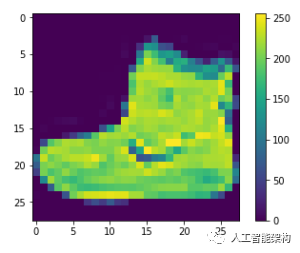
预处理数据
1plt.figure()2plt.imshow(train_images[0])3plt.colorbar()4plt.grid(False)5plt.show()6#If you inspect the first image in the training set, you will see that the pixel values fall in the range of 0 to 255.
2plt.imshow(train_images[0])
3plt.colorbar()
4plt.grid(False)
5plt.show()
6#If you inspect the first image in the training set, you will see that the pixel values fall in the range of 0 to 255.
缩放0-1图像,将其输入神经网络
1train_images = train_images / 255.02test_images = test_images / 255.0255.0
2test_images = test_images / 255.0
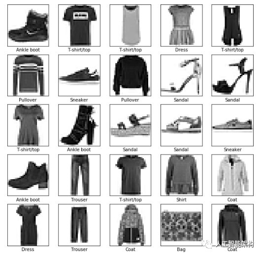
显示部分图像
 1plt.figure(figsize=(10,10)) 2for i in range(25): 3    plt.subplot(5,5,i+1) 4    plt.xticks([]) 5    plt.yticks([]) 6    plt.grid(False) 7    plt.imshow(train_images[i], cmap=plt.cm.binary) 8    plt.xlabel(class_names[train_labels[i]]) 9plt.show()1010,10))
 2for i in range(25):
 3    plt.subplot(5,5,i+1)
 4    plt.xticks([])
 5    plt.yticks([])
 6    plt.grid(False)
 7    plt.imshow(train_images[i], cmap=plt.cm.binary)
 8    plt.xlabel(class_names[train_labels[i]])
 9plt.show()
10
设置层
1model = keras.Sequential([2    keras.layers.Flatten(input_shape=(28, 28)),3    keras.layers.Dense(128, activation=tf.nn.relu),4    keras.layers.Dense(10, activation=tf.nn.softmax)5])
2    keras.layers.Flatten(input_shape=(28, 28)),
3    keras.layers.Dense(128, activation=tf.nn.relu),
4    keras.layers.Dense(10, activation=tf.nn.softmax)
5])
编译模型
1model.compile(optimizer='adam',2              loss='sparse_categorical_crossentropy',3              metrics=['accuracy'])'adam',
2              loss='sparse_categorical_crossentropy',
3              metrics=['accuracy'])
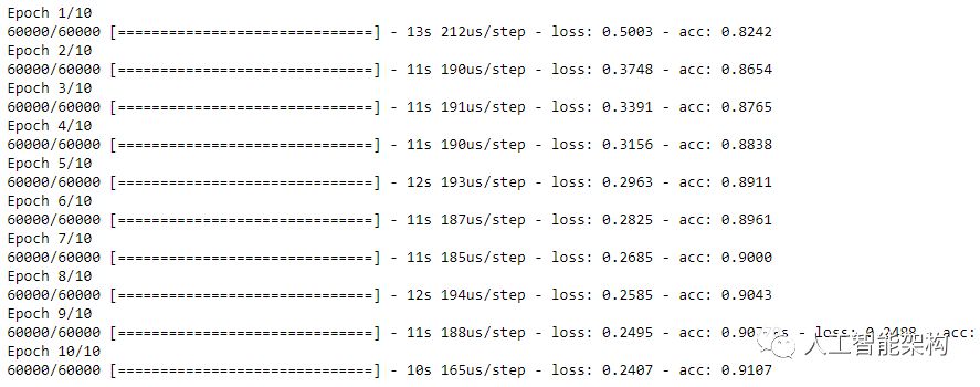
模型训练
1model.fit(train_images, train_labels, epochs=10)10)
评估准确性
1test_loss, test_acc = model.evaluate(test_images, test_labels)2print('Test accuracy:', test_acc)
2print('Test accuracy:', test_acc)

预测
1predictions = model.predict(test_images)2predictions[0]
2predictions[0]
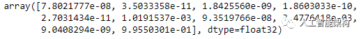
预测结果是10个数字的数组,即对应于图像的10种不同服装中的每一种。我们可以看到哪个标签具有最高的置信度值。
1np.argmax(predictions[0])2#Model is most confident that it's an ankle boot. Let's see if it's correct30])
2#Model is most confident that it's an ankle boot. Let's see if it's correct
3
输出:9
1test_labels[0]0]
查看10个全集
 1def plot_image(i, predictions_array, true_label, img): 2  predictions_array, true_label, img = predictions_array[i], true_label[i], img[i] 3  plt.grid(False) 4  plt.xticks([]) 5  plt.yticks([]) 6  plt.imshow(img, cmap=plt.cm.binary) 7  predicted_label = np.argmax(predictions_array) 8  if predicted_label == true_label: 9    color = 'green'10  else:11    color = 'red'12  plt.xlabel("{} {:2.0f}% ({})".format(class_names[predicted_label],13                                100*np.max(predictions_array),14                                class_names[true_label]),15                                color=color)16def plot_value_array(i, predictions_array, true_label):17  predictions_array, true_label = predictions_array[i], true_label[i]18  plt.grid(False)19  plt.xticks([])20  plt.yticks([])21  thisplot = plt.bar(range(10), predictions_array, color="#777777")22  plt.ylim([0, 1])23  predicted_label = np.argmax(predictions_array)24  thisplot[predicted_label].set_color('red')25  thisplot[true_label].set_color('green')def plot_image(i, predictions_array, true_label, img):
 2  predictions_array, true_label, img = predictions_array[i], true_label[i], img[i]
 3  plt.grid(False)
 4  plt.xticks([])
 5  plt.yticks([])
 6  plt.imshow(img, cmap=plt.cm.binary)
 7  predicted_label = np.argmax(predictions_array)
 8  if predicted_label == true_label:
 9    color = 'green'
10  else:
11    color = 'red'
12  plt.xlabel("{} {:2.0f}% ({})".format(class_names[predicted_label],
13                                100*np.max(predictions_array),
14                                class_names[true_label]),
15                                color=color)
16def plot_value_array(i, predictions_array, true_label):
17  predictions_array, true_label = predictions_array[i], true_label[i]
18  plt.grid(False)
19  plt.xticks([])
20  plt.yticks([])
21  thisplot = plt.bar(range(10), predictions_array, color="#777777")
22  plt.ylim([0, 1])
23  predicted_label = np.argmax(predictions_array)
24  thisplot[predicted_label].set_color('red')
25  thisplot[true_label].set_color('green')
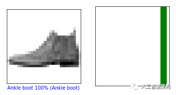
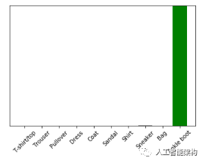
第0张和第10张图片
1i = 02plt.figure(figsize=(6,3))3plt.subplot(1,2,1)4plot_image(i, predictions, test_labels, test_images)5plt.subplot(1,2,2)6plot_value_array(i, predictions,  test_labels)7plt.show()0
2plt.figure(figsize=(6,3))
3plt.subplot(1,2,1)
4plot_image(i, predictions, test_labels, test_images)
5plt.subplot(1,2,2)
6plot_value_array(i, predictions,  test_labels)
7plt.show()
1i = 102plt.figure(figsize=(6,3))3plt.subplot(1,2,1)4plot_image(i, predictions, test_labels, test_images)5plt.subplot(1,2,2)6plot_value_array(i, predictions,  test_labels)7plt.show()10
2plt.figure(figsize=(6,3))
3plt.subplot(1,2,1)
4plot_image(i, predictions, test_labels, test_images)
5plt.subplot(1,2,2)
6plot_value_array(i, predictions,  test_labels)
7plt.show()
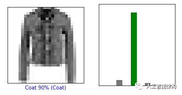
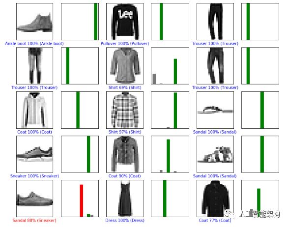
绘制几幅图像进行预测。正确为绿色,不正确为红色
 1num_rows = 5 2num_cols = 3 3num_images = num_rows*num_cols 4plt.figure(figsize=(2*2*num_cols, 2*num_rows)) 5for i in range(num_images): 6  plt.subplot(num_rows, 2*num_cols, 2*i+1) 7  plot_image(i, predictions, test_labels, test_images) 8  plt.subplot(num_rows, 2*num_cols, 2*i+2) 9  plot_value_array(i, predictions, test_labels)10plt.show()5
 2num_cols = 3
 3num_images = num_rows*num_cols
 4plt.figure(figsize=(2*2*num_cols, 2*num_rows))
 5for i in range(num_images):
 6  plt.subplot(num_rows, 2*num_cols, 2*i+1)
 7  plot_image(i, predictions, test_labels, test_images)
 8  plt.subplot(num_rows, 2*num_cols, 2*i+2)
 9  plot_value_array(i, predictions, test_labels)
10plt.show()
使用训练的模型对单个图像进行预测
 1# Grab an image from the test dataset 2img = test_images[0] 3 4print(img.shape) 5 6# Add the image to a batch where it's the only member. 7img = (np.expand_dims(img,0)) 8 9print(img.shape)1011predictions_single = model.predict(img) 12print(predictions_single)# Grab an image from the test dataset
 2img = test_images[0]
 3
 4print(img.shape)
 5
 6# Add the image to a batch where it's the only member.
 7img = (np.expand_dims(img,0))
 8
 9print(img.shape)
10
11predictions_single = model.predict(img)
12print(predictions_single)

1plot_value_array(0, predictions_single, test_labels)2plt.xticks(range(10), class_names, rotation=45)3plt.show()0, predictions_single, test_labels)
2plt.xticks(range(10), class_names, rotation=45)
3plt.show()
批量处理唯一图像的预测
1prediction_result = np.argmax(predictions_single[0])0])
CIFAR-10: CNN
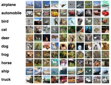
CIFAR-10数据集由飞机、狗、猫和其他物体组成。对图像进行预处理,然后在所有样本上训练卷积神经网络。需要对图像进行标准化。通过这个用例肯定能解释你曾经对TensorFlow图像分类的疑虑。
下载数据
 1from urllib.request import urlretrieve 2from os.path import isfile, isdir 3from tqdm import tqdm  4import tarfile 5cifar10_dataset_folder_path = 'cifar-10-batches-py' 6class DownloadProgress(tqdm): 7    last_block = 0 8    def hook(self, block_num=1, block_size=1, total_size=None): 9        self.total = total_size10        self.update((block_num - self.last_block) * block_size)11        self.last_block = block_num12""" 13    check if the data (zip) file is already downloaded14    if not, download it from "https://www.cs.toronto.edu/~kriz/cifar-10-python.tar.gz" and save as cifar-10-python.tar.gz15"""16if not isfile('cifar-10-python.tar.gz'):17    with DownloadProgress(unit='B', unit_scale=True, miniters=1, desc='CIFAR-10 Dataset') as pbar:18        urlretrieve(19            'https://www.cs.toronto.edu/~kriz/cifar-10-python.tar.gz',20            'cifar-10-python.tar.gz',21            pbar.hook)22if not isdir(cifar10_dataset_folder_path):23    with tarfile.open('cifar-10-python.tar.gz') as tar:24        tar.extractall()25        tar.close()from urllib.request import urlretrieve
 2from os.path import isfile, isdir
 3from tqdm import tqdm
 4import tarfile
 5cifar10_dataset_folder_path = 'cifar-10-batches-py'
 6class DownloadProgress(tqdm):
 7    last_block = 0
 8    def hook(self, block_num=1, block_size=1, total_size=None):
 9        self.total = total_size
10        self.update((block_num - self.last_block) * block_size)
11        self.last_block = block_num
12"""
13    check if the data (zip) file is already downloaded
14    if not, download it from "https://www.cs.toronto.edu/~kriz/cifar-10-python.tar.gz" and save as cifar-10-python.tar.gz
15"""
16if not isfile('cifar-10-python.tar.gz'):
17    with DownloadProgress(unit='B', unit_scale=True, miniters=1, desc='CIFAR-10 Dataset') as pbar:
18        urlretrieve(
19            'https://www.cs.toronto.edu/~kriz/cifar-10-python.tar.gz',
20            'cifar-10-python.tar.gz',
21            pbar.hook)
22if not isdir(cifar10_dataset_folder_path):
23    with tarfile.open('cifar-10-python.tar.gz') as tar:
24        tar.extractall()
25        tar.close()
导入必要的库
1import pickle2import numpy as np3import matplotlib.pyplot as pltimport pickle
2import numpy as np
3import matplotlib.pyplot as plt
了解数据
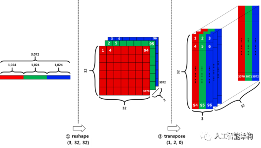
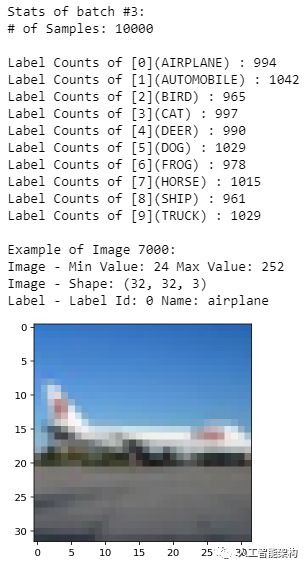
原始数据批量为10000*3072张,用numpy数组表示,其中10000是样本数据的数量。图像时彩色的,尺寸为32*32.可以(width x height x num_channel)或(num_channel x width x height)的格式进行输入。我们定义标签。
重塑数据
将分为两个阶段重塑数据。
首先,将行向量(3072)分成3个。每个部分对应于每个通道,维度将是3*1024.然后将上一步的结果除以32,这里的32是图像的宽度,则将为3*32*32.
其次,我们必须将数据从(num_channel,width,height)转置为(width,height,num_channel)。使用转置函数。
1def load_cfar10_batch(cifar10_dataset_folder_path, batch_id):2    with open(cifar10_dataset_folder_path + '/data_batch_' + str(batch_id), mode='rb') as file:3        # note the encoding type is 'latin1'4        batch = pickle.load(file, encoding='latin1')5    features = batch['data'].reshape((len(batch['data']), 3, 32, 32)).transpose(0, 2, 3, 1)6    labels = batch['labels']7    return features, labeldef load_cfar10_batch(cifar10_dataset_folder_path, batch_id):
2    with open(cifar10_dataset_folder_path + '/data_batch_' + str(batch_id), mode='rb') as file:
3        # note the encoding type is 'latin1'
4        batch = pickle.load(file, encoding='latin1')
5    features = batch['data'].reshape((len(batch['data']), 3, 32, 32)).transpose(0, 2, 3, 1)
6    labels = batch['labels']
7    return features, label
探索数据
1%matplotlib inline2%config InlineBackend.figure_format = 'retina'3import numpy as np4# Explore the dataset5batch_id = 36sample_id = 70007display_stats(cifar10_dataset_folder_path, batch_id, sample_id)
2%config InlineBackend.figure_format = 'retina'
3import numpy as np
4# Explore the dataset
5batch_id = 3
6sample_id = 7000
7display_stats(cifar10_dataset_folder_path, batch_id, sample_id)
实现预处理功能
通过Min-Max Normalization标准化数据。可以简单的是所有x值的范围在0和1之间。
y = (x-min) / (max-min)
编码
 1def one_hot_encode(x): 2    """ 3        argument 4            - x: a list of labels 5        return 6            - one hot encoding matrix (number of labels, number of class) 7    """ 8    encoded = np.zeros((len(x), 10)) 9    for idx, val in enumerate(x):10        encoded[idx][val] = 111    return encodeddef one_hot_encode(x):
 2    """
 3        argument
 4            - x: a list of labels
 5        return
 6            - one hot encoding matrix (number of labels, number of class)
 7    """
 8    encoded = np.zeros((len(x), 10))
 9    for idx, val in enumerate(x):
10        encoded[idx][val] = 1
11    return encoded
预处理和保存数据
 1def _preprocess_and_save(normalize, one_hot_encode, features, labels, filename): 2    features = normalize(features) 3    labels = one_hot_encode(labels) 4    pickle.dump((features, labels), open(filename, 'wb')) 5def preprocess_and_save_data(cifar10_dataset_folder_path, normalize, one_hot_encode): 6    n_batches = 5 7    valid_features = [] 8    valid_labels = [] 9    for batch_i in range(1, n_batches + 1):10        features, labels = load_cfar10_batch(cifar10_dataset_folder_path, batch_i)11        # find index to be the point as validation data in the whole dataset of the batch (10%)12        index_of_validation = int(len(features) * 0.1)13        # preprocess the 90% of the whole dataset of the batch14        # - normalize the features15        # - one_hot_encode the lables16        # - save in a new file named, "preprocess_batch_" + batch_number17        # - each file for each batch18        _preprocess_and_save(normalize, one_hot_encode,19                             features[:-index_of_validation], labels[:-index_of_validation], 20                             'preprocess_batch_' + str(batch_i) + '.p')21        # unlike the training dataset, validation dataset will be added through all batch dataset22        # - take 10% of the whold dataset of the batch23        # - add them into a list of24        #   - valid_features25        #   - valid_labels26        valid_features.extend(features[-index_of_validation:])27        valid_labels.extend(labels[-index_of_validation:])28    # preprocess the all stacked validation dataset29    _preprocess_and_save(normalize, one_hot_encode,30                         np.array(valid_features), np.array(valid_labels),31                         'preprocess_validation.p')32    # load the test dataset33    with open(cifar10_dataset_folder_path + '/test_batch', mode='rb') as file:34        batch = pickle.load(file, encoding='latin1')35    # preprocess the testing data36    test_features = batch['data'].reshape((len(batch['data']), 3, 32, 32)).transpose(0, 2, 3, 1)37    test_labels = batch['labels']38    # Preprocess and Save all testing data39    _preprocess_and_save(normalize, one_hot_encode,40                         np.array(test_features), np.array(test_labels),41                         'preprocess_training.p')def _preprocess_and_save(normalize, one_hot_encode, features, labels, filename):
 2    features = normalize(features)
 3    labels = one_hot_encode(labels)
 4    pickle.dump((features, labels), open(filename, 'wb'))
 5def preprocess_and_save_data(cifar10_dataset_folder_path, normalize, one_hot_encode):
 6    n_batches = 5
 7    valid_features = []
 8    valid_labels = []
 9    for batch_i in range(1, n_batches + 1):
10        features, labels = load_cfar10_batch(cifar10_dataset_folder_path, batch_i)
11        # find index to be the point as validation data in the whole dataset of the batch (10%)
12        index_of_validation = int(len(features) * 0.1)
13        # preprocess the 90% of the whole dataset of the batch
14        # - normalize the features
15        # - one_hot_encode the lables
16        # - save in a new file named, "preprocess_batch_" + batch_number
17        # - each file for each batch
18        _preprocess_and_save(normalize, one_hot_encode,
19                             features[:-index_of_validation], labels[:-index_of_validation],
20                             'preprocess_batch_' + str(batch_i) + '.p')
21        # unlike the training dataset, validation dataset will be added through all batch dataset
22        # - take 10% of the whold dataset of the batch
23        # - add them into a list of
24        #   - valid_features
25        #   - valid_labels
26        valid_features.extend(features[-index_of_validation:])
27        valid_labels.extend(labels[-index_of_validation:])
28    # preprocess the all stacked validation dataset
29    _preprocess_and_save(normalize, one_hot_encode,
30                         np.array(valid_features), np.array(valid_labels),
31                         'preprocess_validation.p')
32    # load the test dataset
33    with open(cifar10_dataset_folder_path + '/test_batch', mode='rb') as file:
34        batch = pickle.load(file, encoding='latin1')
35    # preprocess the testing data
36    test_features = batch['data'].reshape((len(batch['data']), 3, 32, 32)).transpose(0, 2, 3, 1)
37    test_labels = batch['labels']
38    # Preprocess and Save all testing data
39    _preprocess_and_save(normalize, one_hot_encode,
40                         np.array(test_features), np.array(test_labels),
41                         'preprocess_training.p')
建立网络
整个模型共有14层。

 1import tensorflow as tf 2def conv_net(x, keep_prob): 3    conv1_filter = tf.Variable(tf.truncated_normal(shape=[3, 3, 3, 64], mean=0, stddev=0.08)) 4    conv2_filter = tf.Variable(tf.truncated_normal(shape=[3, 3, 64, 128], mean=0, stddev=0.08)) 5    conv3_filter = tf.Variable(tf.truncated_normal(shape=[5, 5, 128, 256], mean=0, stddev=0.08)) 6    conv4_filter = tf.Variable(tf.truncated_normal(shape=[5, 5, 256, 512], mean=0, stddev=0.08)) 7    # 1, 2 8    conv1 = tf.nn.conv2d(x, conv1_filter, strides=[1,1,1,1], padding='SAME') 9    conv1 = tf.nn.relu(conv1)10    conv1_pool = tf.nn.max_pool(conv1, ksize=[1,2,2,1], strides=[1,2,2,1], padding='SAME')11    conv1_bn = tf.layers.batch_normalization(conv1_pool)12    # 3, 413    conv2 = tf.nn.conv2d(conv1_bn, conv2_filter, strides=[1,1,1,1], padding='SAME')14    conv2 = tf.nn.relu(conv2)15    conv2_pool = tf.nn.max_pool(conv2, ksize=[1,2,2,1], strides=[1,2,2,1], padding='SAME')    16    conv2_bn = tf.layers.batch_normalization(conv2_pool)17    # 5, 618    conv3 = tf.nn.conv2d(conv2_bn, conv3_filter, strides=[1,1,1,1], padding='SAME')19    conv3 = tf.nn.relu(conv3)20    conv3_pool = tf.nn.max_pool(conv3, ksize=[1,2,2,1], strides=[1,2,2,1], padding='SAME')  21    conv3_bn = tf.layers.batch_normalization(conv3_pool)22    # 7, 823    conv4 = tf.nn.conv2d(conv3_bn, conv4_filter, strides=[1,1,1,1], padding='SAME')24    conv4 = tf.nn.relu(conv4)25    conv4_pool = tf.nn.max_pool(conv4, ksize=[1,2,2,1], strides=[1,2,2,1], padding='SAME')26    conv4_bn = tf.layers.batch_normalization(conv4_pool)27    # 928    flat = tf.contrib.layers.flatten(conv4_bn)  29    # 1030    full1 = tf.contrib.layers.fully_connected(inputs=flat, num_outputs=128, activation_fn=tf.nn.relu)31    full1 = tf.nn.dropout(full1, keep_prob)32    full1 = tf.layers.batch_normalization(full1)33    # 1134    full2 = tf.contrib.layers.fully_connected(inputs=full1, num_outputs=256, activation_fn=tf.nn.relu)35    full2 = tf.nn.dropout(full2, keep_prob)36    full2 = tf.layers.batch_normalization(full2)37    # 1238    full3 = tf.contrib.layers.fully_connected(inputs=full2, num_outputs=512, activation_fn=tf.nn.relu)39    full3 = tf.nn.dropout(full3, keep_prob)40    full3 = tf.layers.batch_normalization(full3)    41    # 1342    full4 = tf.contrib.layers.fully_connected(inputs=full3, num_outputs=1024, activation_fn=tf.nn.relu)43    full4 = tf.nn.dropout(full4, keep_prob)44    full4 = tf.layers.batch_normalization(full4)        45    # 1446    out = tf.contrib.layers.fully_connected(inputs=full3, num_outputs=10, activation_fn=None)47    return outimport tensorflow as tf
 2def conv_net(x, keep_prob):
 3    conv1_filter = tf.Variable(tf.truncated_normal(shape=[3, 3, 3, 64], mean=0, stddev=0.08))
 4    conv2_filter = tf.Variable(tf.truncated_normal(shape=[3, 3, 64, 128], mean=0, stddev=0.08))
 5    conv3_filter = tf.Variable(tf.truncated_normal(shape=[5, 5, 128, 256], mean=0, stddev=0.08))
 6    conv4_filter = tf.Variable(tf.truncated_normal(shape=[5, 5, 256, 512], mean=0, stddev=0.08))
 7    # 1, 2
 8    conv1 = tf.nn.conv2d(x, conv1_filter, strides=[1,1,1,1], padding='SAME')
 9    conv1 = tf.nn.relu(conv1)
10    conv1_pool = tf.nn.max_pool(conv1, ksize=[1,2,2,1], strides=[1,2,2,1], padding='SAME')
11    conv1_bn = tf.layers.batch_normalization(conv1_pool)
12    # 3, 4
13    conv2 = tf.nn.conv2d(conv1_bn, conv2_filter, strides=[1,1,1,1], padding='SAME')
14    conv2 = tf.nn.relu(conv2)
15    conv2_pool = tf.nn.max_pool(conv2, ksize=[1,2,2,1], strides=[1,2,2,1], padding='SAME')
16    conv2_bn = tf.layers.batch_normalization(conv2_pool)
17    # 5, 6
18    conv3 = tf.nn.conv2d(conv2_bn, conv3_filter, strides=[1,1,1,1], padding='SAME')
19    conv3 = tf.nn.relu(conv3)
20    conv3_pool = tf.nn.max_pool(conv3, ksize=[1,2,2,1], strides=[1,2,2,1], padding='SAME')
21    conv3_bn = tf.layers.batch_normalization(conv3_pool)
22    # 7, 8
23    conv4 = tf.nn.conv2d(conv3_bn, conv4_filter, strides=[1,1,1,1], padding='SAME')
24    conv4 = tf.nn.relu(conv4)
25    conv4_pool = tf.nn.max_pool(conv4, ksize=[1,2,2,1], strides=[1,2,2,1], padding='SAME')
26    conv4_bn = tf.layers.batch_normalization(conv4_pool)
27    # 9
28    flat = tf.contrib.layers.flatten(conv4_bn)
29    # 10
30    full1 = tf.contrib.layers.fully_connected(inputs=flat, num_outputs=128, activation_fn=tf.nn.relu)
31    full1 = tf.nn.dropout(full1, keep_prob)
32    full1 = tf.layers.batch_normalization(full1)
33    # 11
34    full2 = tf.contrib.layers.fully_connected(inputs=full1, num_outputs=256, activation_fn=tf.nn.relu)
35    full2 = tf.nn.dropout(full2, keep_prob)
36    full2 = tf.layers.batch_normalization(full2)
37    # 12
38    full3 = tf.contrib.layers.fully_connected(inputs=full2, num_outputs=512, activation_fn=tf.nn.relu)
39    full3 = tf.nn.dropout(full3, keep_prob)
40    full3 = tf.layers.batch_normalization(full3)
41    # 13
42    full4 = tf.contrib.layers.fully_connected(inputs=full3, num_outputs=1024, activation_fn=tf.nn.relu)
43    full4 = tf.nn.dropout(full4, keep_prob)
44    full4 = tf.layers.batch_normalization(full4)
45    # 14
46    out = tf.contrib.layers.fully_connected(inputs=full3, num_outputs=10, activation_fn=None)
47    return out
超参数
1epochs = 102batch_size = 1283keep_probability = 0.74learning_rate = 0.00110
2batch_size = 128
3keep_probability = 0.7
4learning_rate = 0.001
1logits = conv_net(x, keep_prob)2model = tf.identity(logits, name='logits') # Name logits Tensor, so that can be loaded from disk after training3# Loss and Optimizer4cost = tf.reduce_mean(tf.nn.softmax_cross_entropy_with_logits(logits=logits, labels=y))5optimizer = tf.train.AdamOptimizer(learning_rate=learning_rate).minimize(cost)6# Accuracy7correct_pred = tf.equal(tf.argmax(logits, 1), tf.argmax(y, 1))8accuracy = tf.reduce_mean(tf.cast(correct_pred, tf.float32), name='accuracy')
2model = tf.identity(logits, name='logits') # Name logits Tensor, so that can be loaded from disk after training
3# Loss and Optimizer
4cost = tf.reduce_mean(tf.nn.softmax_cross_entropy_with_logits(logits=logits, labels=y))
5optimizer = tf.train.AdamOptimizer(learning_rate=learning_rate).minimize(cost)
6# Accuracy
7correct_pred = tf.equal(tf.argmax(logits, 1), tf.argmax(y, 1))
8accuracy = tf.reduce_mean(tf.cast(correct_pred, tf.float32), name='accuracy')
训练神经网络
1#Single Optimizationdef train_neural_network(session, optimizer, keep_probability, feature_batch, label_batch):2    session.run(optimizer, 3                feed_dict={4                    x: feature_batch,5                    y: label_batch,6                    keep_prob: keep_probability7                })#Single Optimizationdef train_neural_network(session, optimizer, keep_probability, feature_batch, label_batch):
2    session.run(optimizer,
3                feed_dict={

4                    x: feature_batch,
5                    y: label_batch,
6                    keep_prob: keep_probability
7                })
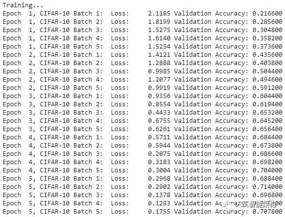
 1#Showing Stats 2def print_stats(session, feature_batch, label_batch, cost, accuracy): 3    loss = sess.run(cost,  4                    feed_dict={ 5                        x: feature_batch, 6                        y: label_batch, 7                        keep_prob: 1. 8                    }) 9    valid_acc = sess.run(accuracy, 10                         feed_dict={11                             x: valid_features,12                             y: valid_labels,13                             keep_prob: 1.14                         })15    print('Loss: {:>10.4f} Validation Accuracy: {:.6f}'.format(loss, valid_acc))#Showing Stats
 2def print_stats(session, feature_batch, label_batch, cost, accuracy):
 3    loss = sess.run(cost,
 4                    feed_dict={

 5                        x: feature_batch,
 6                        y: label_batch,
 7                        keep_prob: 1.
 8                    })
 9    valid_acc = sess.run(accuracy,
10                         feed_dict={

11                             x: valid_features,
12                             y: valid_labels,
13                             keep_prob: 1.
14                         })
15    print('Loss: {:>10.4f} Validation Accuracy: {:.6f}'.format(loss, valid_acc))
全面训练和保存模型
 1def batch_features_labels(features, labels, batch_size): 2    """ 3    Split features and labels into batches 4    """ 5    for start in range(0, len(features), batch_size): 6        end = min(start + batch_size, len(features)) 7        yield features[start:end], labels[start:end] 8def load_preprocess_training_batch(batch_id, batch_size): 9    """10    Load the Preprocessed Training data and return them in batches of <batch_size> or less11    """12    filename = 'preprocess_batch_' + str(batch_id) + '.p'13    features, labels = pickle.load(open(filename, mode='rb'))14    # Return the training data in batches of size <batch_size> or less15    return batch_features_labels(features, labels, batch_size)def batch_features_labels(features, labels, batch_size):
 2    """
 3    Split features and labels into batches
 4    """
 5    for start in range(0, len(features), batch_size):
 6        end = min(start + batch_size, len(features))
 7        yield features[start:end], labels[start:end]
 8def load_preprocess_training_batch(batch_id, batch_size):
 9    """
10    Load the Preprocessed Training data and return them in batches of <batch_size> or less
11    """
12    filename = 'preprocess_batch_' + str(batch_id) + '.p'
13    features, labels = pickle.load(open(filename, mode='rb'))
14    # Return the training data in batches of size <batch_size> or less
15    return batch_features_labels(features, labels, batch_size)
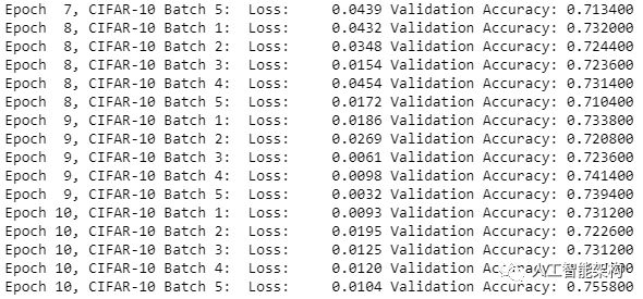
 1#Saving Model and Pathsave_model_path = './image_classification' 2print('Training...') 3with tf.Session() as sess: 4    # Initializing the variables 5    sess.run(tf.global_variables_initializer()) 6    # Training cycle 7    for epoch in range(epochs): 8        # Loop over all batches 9        n_batches = 510        for batch_i in range(1, n_batches + 1):11            for batch_features, batch_labels in load_preprocess_training_batch(batch_i, batch_size):12                train_neural_network(sess, optimizer, keep_probability, batch_features, batch_labels)13            print('Epoch {:>2}, CIFAR-10 Batch {}:  '.format(epoch + 1, batch_i), end='')14            print_stats(sess, batch_features, batch_labels, cost, accuracy)#Saving Model and Pathsave_model_path = './image_classification'
 2print('Training...')
 3with tf.Session() as sess:
 4    # Initializing the variables
 5    sess.run(tf.global_variables_initializer())
 6    # Training cycle
 7    for epoch in range(epochs):
 8        # Loop over all batches
 9        n_batches = 5
10        for batch_i in range(1, n_batches + 1):
11            for batch_features, batch_labels in load_preprocess_training_batch(batch_i, batch_size):
12                train_neural_network(sess, optimizer, keep_probability, batch_features, batch_labels)
13            print('Epoch {:>2}, CIFAR-10 Batch {}:  '.format(epoch + 1, batch_i), end='')
14            print_stats(sess, batch_features, batch_labels, cost, accuracy)
1# Save Model2    saver = tf.train.Saver()3    save_path = saver.save(sess, save_model_path)# Save Model
2    saver = tf.train.Saver()
3    save_path = saver.save(sess, save_model_path)
现在,TensorFlow图像分类的重要部分已经完成了,接着该测试模型。
测试模型
1import pickle 2import numpy as np 3import matplotlib.pyplot as plt 4from sklearn.preprocessing import LabelBinarizer 5def batch_features_labels(features, labels, batch_size): 6 """ 7 Split features and labels into batches 8 """ 9 for start in range(0, len(features), batch_size):10 end = min(start + batch_size, len(features))11 yield features[start:end], labels[start:end]12def display_image_predictions(features, labels, predictions, top_n_predictions):13 n_classes = 1014 label_names = load_label_names()15 label_binarizer = LabelBinarizer()16 label_binarizer.fit(range(n_classes))17 label_ids = label_binarizer.inverse_transform(np.array(labels))18 fig, axies = plt.subplots(nrows=top_n_predictions, ncols=2, figsize=(20, 10))19 fig.tight_layout()20 fig.suptitle('Softmax Predictions', fontsize=20, y=1.1)21 n_predictions = 322 margin = 0.0523 ind = np.arange(n_predictions)24 width = (1. - 2. * margin) / n_predictions25 for image_i, (feature, label_id, pred_indicies, pred_values) in enumerate(zip(features, label_ids, predictions.indices, predictions.values)):26 if (image_i < top_n_predictions):27 pred_names = [label_names[pred_i] for pred_i in pred_indicies]28 correct_name = label_names[label_id]29 axies[image_i][0].imshow((feature*255).astype(np.int32, copy=False))30 axies[image_i][0].set_title(correct_name)31 axies[image_i][0].set_axis_off()32 axies[image_i][1].barh(ind + margin, pred_values[:3], width)33 axies[image_i][1].set_yticks(ind + margin)34 axies[image_i][1].set_yticklabels(pred_names[::-1])35 axies[image_i][1].set_xticks([0, 0.5, 1.0])import pickle
2import numpy as np
3import matplotlib.pyplot as plt
4from sklearn.preprocessing import LabelBinarizer
5def batch_features_labels(features, labels, batch_size):
6 """
7 Split features and labels into batches
8 """
9 for start in range(0, len(features), batch_size):
10 end = min(start + batch_size, len(features))
11 yield features[start:end], labels[start:end]
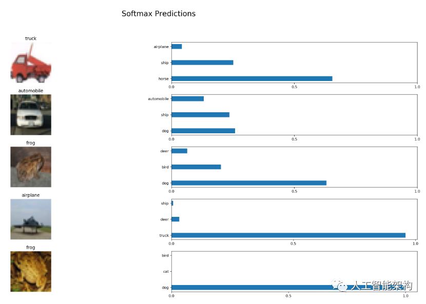
12def display_image_predictions(features, labels, predictions, top_n_predictions):
13 n_classes = 10
14 label_names = load_label_names()
15 label_binarizer = LabelBinarizer()
16 label_binarizer.fit(range(n_classes))
17 label_ids = label_binarizer.inverse_transform(np.array(labels))
18 fig, axies = plt.subplots(nrows=top_n_predictions, ncols=2, figsize=(20, 10))
19 fig.tight_layout()
20 fig.suptitle('Softmax Predictions', fontsize=20, y=1.1)
21 n_predictions = 3
22 margin = 0.05
23 ind = np.arange(n_predictions)
24 width = (1. - 2. * margin) / n_predictions
25 for image_i, (feature, label_id, pred_indicies, pred_values) in enumerate(zip(features, label_ids, predictions.indices, predictions.values)):
26 if (image_i < top_n_predictions):
27 pred_names = [label_names[pred_i] for pred_i in pred_indicies]
28 correct_name = label_names[label_id]
29 axies[image_i][0].imshow((feature*255).astype(np.int32, copy=False))
30 axies[image_i][0].set_title(correct_name)
31 axies[image_i][0].set_axis_off()
32 axies[image_i][1].barh(ind + margin, pred_values[:3], width)
33 axies[image_i][1].set_yticks(ind + margin)
34 axies[image_i][1].set_yticklabels(pred_names[::-1])
35 axies[image_i][1].set_xticks([0, 0.5, 1.0])
 1%matplotlib inline 2%config InlineBackend.figure_format = 'retina' 3import tensorflow as tf 4import pickle 5import random 6save_model_path = './image_classification' 7batch_size = 64 8n_samples = 10 9top_n_predictions = 510def test_model():11    test_features, test_labels = pickle.load(open('preprocess_training.p', mode='rb'))12    loaded_graph = tf.Graph()13    with tf.Session(graph=loaded_graph) as sess:14        # Load model15        loader = tf.train.import_meta_graph(save_model_path + '.meta')16        loader.restore(sess, save_model_path)
 2%config InlineBackend.figure_format = 'retina'
 3import tensorflow as tf
 4import pickle
 5import random
 6save_model_path = './image_classification'
 7batch_size = 64
 8n_samples = 10
 9top_n_predictions = 5
10def test_model():
11    test_features, test_labels = pickle.load(open('preprocess_training.p', mode='rb'))
12    loaded_graph = tf.Graph()
13    with tf.Session(graph=loaded_graph) as sess:
14        # Load model
15        loader = tf.train.import_meta_graph(save_model_path + '.meta')
16        loader.restore(sess, save_model_path)
1# Get Tensors from loaded model2        loaded_x = loaded_graph.get_tensor_by_name('input_x:0')3        loaded_y = loaded_graph.get_tensor_by_name('output_y:0')4        loaded_keep_prob = loaded_graph.get_tensor_by_name('keep_prob:0')5        loaded_logits = loaded_graph.get_tensor_by_name('logits:0')6        loaded_acc = loaded_graph.get_tensor_by_name('accuracy:0')# Get Tensors from loaded model
2        loaded_x = loaded_graph.get_tensor_by_name('input_x:0')
3        loaded_y = loaded_graph.get_tensor_by_name('output_y:0')
4        loaded_keep_prob = loaded_graph.get_tensor_by_name('keep_prob:0')
5        loaded_logits = loaded_graph.get_tensor_by_name('logits:0')
6        loaded_acc = loaded_graph.get_tensor_by_name('accuracy:0')
1# Get accuracy in batches for memory limitations2        test_batch_acc_total = 03        test_batch_count = 04        for train_feature_batch, train_label_batch in batch_features_labels(test_features, test_labels, batch_size):5            test_batch_acc_total += sess.run(6                loaded_acc,7                feed_dict={loaded_x: train_feature_batch, loaded_y: train_label_batch, loaded_keep_prob: 1.0})8            test_batch_count += 19        print('Testing Accuracy: {}'.format(test_batch_acc_total/test_batch_count))# Get accuracy in batches for memory limitations
2        test_batch_acc_total = 0
3        test_batch_count = 0
4        for train_feature_batch, train_label_batch in batch_features_labels(test_features, test_labels, batch_size):
5            test_batch_acc_total += sess.run(
6                loaded_acc,
7                feed_dict={loaded_x: train_feature_batch, loaded_y: train_label_batch, loaded_keep_prob: 1.0})
8            test_batch_count += 1
9        print('Testing Accuracy: {}
'.format(test_batch_acc_total/test_batch_count))
1# Print Random Samples2        random_test_features, random_test_labels = tuple(zip(*random.sample(list(zip(test_features, test_labels)), n_samples)))3        random_test_predictions = sess.run(4            tf.nn.top_k(tf.nn.softmax(loaded_logits), top_n_predictions),5            feed_dict={loaded_x: random_test_features, loaded_y: random_test_labels, loaded_keep_prob: 1.0})6        display_image_predictions(random_test_features, random_test_labels, random_test_predictions, top_n_predictions)7test_model()# Print Random Samples
2        random_test_features, random_test_labels = tuple(zip(*random.sample(list(zip(test_features, test_labels)), n_samples)))
3        random_test_predictions = sess.run(
4            tf.nn.top_k(tf.nn.softmax(loaded_logits), top_n_predictions),
5            feed_dict={loaded_x: random_test_features, loaded_y: random_test_labels, loaded_keep_prob: 1.0})
6        display_image_predictions(random_test_features, random_test_labels, random_test_predictions, top_n_predictions)
7test_model()
输出测试精度:0.5882762738853503
结语
如果你训练神经网络以获得更多功能,可能会具有更高准确度的结果。通过这个详细的实例,你应该已经可以使用它来分类任何类型的图像了。
长按订阅更多精彩▼

智能推荐
android java.lang.SecurityException: Permission Denial_java.lang.securityexception: permission denial: re-程序员宅基地
文章浏览阅读318次。问题描述:使用adb命令模拟打开APP界面,报异常:原因:<activity android:name=".module_parking.ParkingActivity" android:launchMode="singleTask" android:screenOrientation="landscape"></activity>解决措施:android:..._java.lang.securityexception: permission denial: reading androidx.core.conten
汇编中关于EQU指令的问题 _cont equ $-age汇编指令-程序员宅基地
文章浏览阅读3.1w次,点赞15次,收藏59次。一.COUNT EQU 100;令COUNT的值为100,存储器中为变量分配 0个字节COUNT DB 100 ;令COUNT的值为100,存储器中为变量分配 1个字节COUNT DW 100 ;令COUNT的值为100,存储器中为变量分配 2个字节 count EQU $-ARRA 定义了一个常量,不占用内存单元,代码段中使用它,等价于使用一个立即数。count DW $-ARRA_cont equ $-age汇编指令
Excel 2016新增函数之IFS-程序员宅基地
文章浏览阅读3.2k次。Excel 2016新增函数之IFS在2016年1月功能更新中,EXCEL 2016新增几个常用重要函数,主要有:ifs,switch,maxifs,minifs,concat,textjoin等。注意,要能使用上述函数,Office的版本很重要,并不是所有的Office 2016能使用。建议在https://products.office.com/zh-CN/try试用O..._让excel2016有ifs函数
R语言可视化:散点图与特殊目标样本点标记_r语言中如何在散点图中标记特殊点-程序员宅基地
文章浏览阅读194次。在R语言中,我们可以使用ggplot2包来创建漂亮的散点图,并通过添加特殊目标样本点的标记来进一步凸显它们的重要性。运行以上代码后,我们将获得一个带有特殊目标样本点标记的散点图。这样的可视化方法可以帮助我们更好地理解数据,并凸显出特殊目标样本点在整体数据中的位置和重要性。接下来,我们需要在散点图上添加特殊目标样本点的标记。现在,我们可以使用ggplot2创建散点图,并将特殊目标样本点标记出来。通过运行以上代码,我们可以生成一个带有特殊目标样本点标记的散点图。R语言可视化:散点图与特殊目标样本点标记。_r语言中如何在散点图中标记特殊点
Makefile 之 include_makefile中 include了,源文件没有include-程序员宅基地
文章浏览阅读1.1k次。本节我们讨论如何在一个 Makefile 中包含其它的 makefile 文件。Makefile 中包含其它文件的关键字是“include”,和 C 语言对头文件的包含方式一致。 “include”指示符告诉 make 暂停读取当前的 Makefile,而转去读取“include”指定的一个或者多个文件,完成以后再继续当前 Makefile 的读取。Makefile 中指示符_makefile中 include了,源文件没有include
bluecms 手把手教你0day挖掘-基础入门篇_bluecms找漏洞-程序员宅基地
文章浏览阅读5.2k次。Bluecms后台sql注入漏洞一、环境搭建1、PhP地方门户系统 BlueCMS v1.6 sp1下载地址:https://down.chinaz.com/soft/26181.htm2、PHPstudy apache,mysql集成环境二、代码审计在该cms系统中,其后台存在sql注入漏洞[外链图片转存失败,源站可能有防盗链机制,建议将图片保存下来直接上传(img-wmb7A4Ms-1647335609467)(https://gitee.com/gaohongyu1/csdn/raw/m_bluecms找漏洞
随便推点
水晶报表之图片(插入,显示)_水晶报表显示图片-程序员宅基地
文章浏览阅读4.5k次。工具:Crystal Reports 2008步骤一:打开水晶报表文件,点击上方 插入--->图片(选择文件位置) 接着将图片调整大小后添加到指定位置步骤二:设置图片显示规则,右键选择设置图形格式设置图片格式编辑图片显示规则..._水晶报表显示图片
python连接数据库命令_Mysql-python连接操作数据库-程序员宅基地
文章浏览阅读107次。使用python连接操作数据库--》下载配置python环境--》推荐安装PyMySQL 库:PyMySQL 是一个纯Python 实现的MySQL 客户端操作库,支持事务、存储过程、批量执行等使用命令:pip install pymysql--》连接数据库脚本1 #导入模块2 importpymysql3 #连接数据库4 conn =pymysql.connect(5 host='loc..._python在命令行中连接数据库
9月21日绝地求生服务器维护时间,前沿手游:绝地求生10月21日更新时间 绝地求生10月21日维护到几点...-程序员宅基地
文章浏览阅读448次。非常感谢朋友们点开小编的绝地求生10月21日更新时间 绝地求生10月21日维护到几点文章,因为大家现在都是想要了解到此类的信息,那么既然现在大家都想要知道绝地求生10月21日更新时间 绝地求生10月21日维护到几点,小编今天就来给大家针对这样的问题做个科普介绍吧。我将每天为大家收集和分享一些新鲜又有营养的精彩内容,希望大家能够一如既往的给予小编最大的鼓励和支持,毕竟大家的鼓励和支持才是小编持续更新...
安捷伦Agilent 4395A阻抗分析仪-程序员宅基地
文章浏览阅读332次,点赞10次,收藏6次。评估元件和电路通常需要的增益、相位、群延迟、失真、杂散、CN 和噪声测量可以使用一台仪器进行测量。动态幅度和相位精度为 +/-0.05dB 和 +/-0.3deg。作为频谱分析仪,它的工作频率范围为 10 Hz 至 500 MHz,分辨率带宽 (RBW) 以 1-3-10 步长跨越 1 Hz 至 1 MHz。噪声边带低于 -100 dBc/Hz @ 100 kHz 载波偏移,10 MHz 时灵敏度为 -145 dBm/Hz。+/-0.05 dB /+/-0.3deg 动态幅度/相位精度。
android 文件列表显示,Android: 显示SD卡文件列表-程序员宅基地
文章浏览阅读174次。读取SD卡文件信息,添加到ListView中显示出来:ListView取得SD文件信息的代码:[java]view plaincopy?List>list=newArrayList>();StringsDStateString=Environment.getExternalStorageState();if(sDStateString.equals(Environmen..._android 点击搜索出来的文件后,再点击查看内部文件或sd卡内的文件,这些文件显示一
初学编程需要什么基础,零基础学编程系统化编程课程之编程工具箱文件名称操作构件属性-程序员宅基地
文章浏览阅读66次。初学编程需要什么基础,零基础学编程系统化编程课程之编程工具箱文件名称操作构件属性。上图为 该编程工具构件的基本属性和方法。